1. Introduction

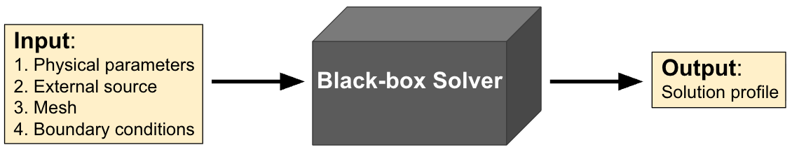
Black-box solvers are systems that are best viewed as versatile solvers that deal with systems of equations without getting into too much mathetmatical detail. They are mostly closed-source solvers that take in equations or scenarios as inputs and give out the solution as an output. For example, you may have a finite element solver that solves the steady-state heat equation depending on the physical parameters (like diffusivity) and the boundary conditions that you input, along with a mesh resolution that you also provide; see Fig. 1. for a diagram showing this process. But to ensure that the solution is accurate on whatever scenario you input, it is important do convergence studies with known manufactured solutions, or at least fine-grid solutions, and most importantly, a test of robustness of the scheme.

The topic of this blog post is to exemplify the importance of verification, validation, and robustness testing when using such black-box solvers, or any solver for that matter. I have personally come across an inordinate amount of reserach articles that present a new solver or numerical scheme, but do not verify or validate their scheme with known solutions, do a thorough analysis of the system, or test for robustness of the system. In such cases, even though you may have convergence of your solver, it is hard to tell if your solution has converged to the ‘right solution’ (if there is a ‘right solution’ in the first place!).

We will build our own solver to solve the elliptic Poisson equation in $1D$

\begin{equation} \label{eq:elliptic_eq} -\frac{d^2 u}{dx^2} = f \text{ in } (0, 1), \; \frac{du}{dx}\bigg\rvert_{x = 0} = \frac{du}{dx}\bigg\rvert_{x=1} = 0, \end{equation}

using the conjugate gradient method and we will show how convergence of our solver does not implicitly imply a physically meaningful solution (although an experienced player may have already guessed the issue at hand!).

2. Computational Solver

We now provide the details of our computational solver. We consider the finite element method to discretize \ref{eq:elliptic_eq} in space and then use the conjugate gradient (CG) method to solve the resulting system of equations.

2.1. Numerical Discretization

We begin by discretizing \ref{eq:elliptic_eq} using $P^1$ Lagrange finite elements (standard Galerkin method). Let $\Omega = (0, 1)$ be divided into $M$ cells $(x_{j}, x_{j+1})$, $0 \leq j \leq M-1$, of uniform width denoted by $h = \frac{1}{M}$. We seek an approximation $u_h \approx u$, with $u_h \in V_h \subset H^1(0, 1)$ such that^{1 2}

\begin{equation} \label{eq:variational_form} \int_{0}^{1} \frac{du_h}{dx} \frac{d\phi}{dx} = \int_{0}^{1} f \phi, \; \forall \phi \in V_h, \end{equation}

where $V_h$ is the subspace of piecewise-linear functions with basis functions given by

By expanding $u_h = \sum_{j=0}^{M} U_j \phi_j$ and choosing $\phi = \phi_j$ in \ref{eq:variational_form} we obtain the discretized system

\begin{equation} \label{eq:linear_system} AU = F, \end{equation}

where $U = [U_0 \; U_1 \; \dots \; U_{M}]^T \in \mathbb{R}^{M+1}$, and $A \in \mathbb{R}^{(M+1)\times (M+1)}$, $F \in \mathbb{R}^{M+1}$ are given by

where we have used the trapezoidal rule to approximate $\int_{0}^{1} f(x)\phi_j(x)dx$ to obtain $F$. Note that the matrix $A$ is symmetric positive semi-definite.

2.2. Linear Solver

The system \ref{eq:linear_system} is linear, symmetric, and can be solved using the CG method ^{3 1}: given $U^{(0)} \in \mathbb{R}^{M+1}$, we set $r^{(0)} = F - A U^{(0)}, \; p^{(0)} = r^{(0)}$, and iterate as follows

For symmetric positive definite matrices, the convergence is guaranteed in $M+1$ iterations (ignoring the round-off error). We iterate the CG algorithm till a prescirbed tolerance $\epsilon$, i.e., we terminate the iteration when

\begin{equation} \lVert (A U^{(m)} - F)^T (A U ^{(m)} - F) \rVert_2 \leq \epsilon. \nonumber \end{equation}

3. Results

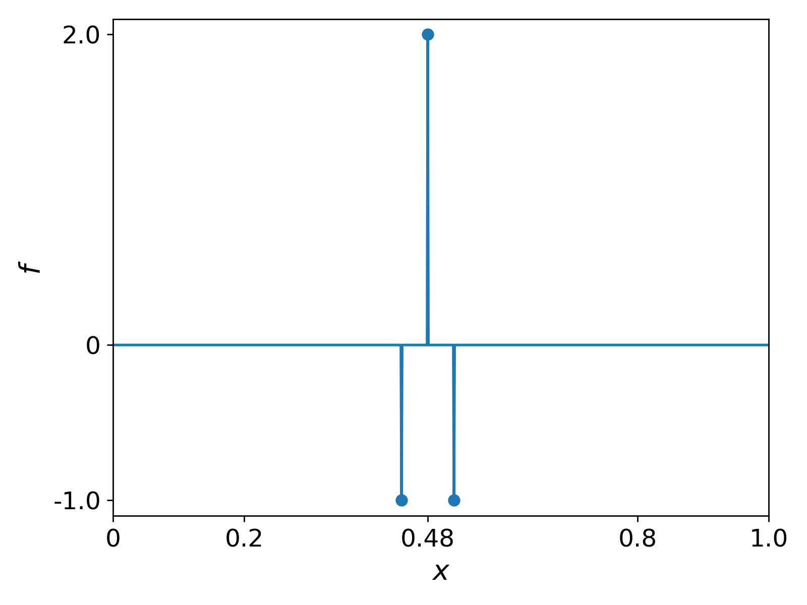
We now use our solver on a given source function $f$. The source $f$ is chosen as to represent a pulse function and is shown in Fig. 2.

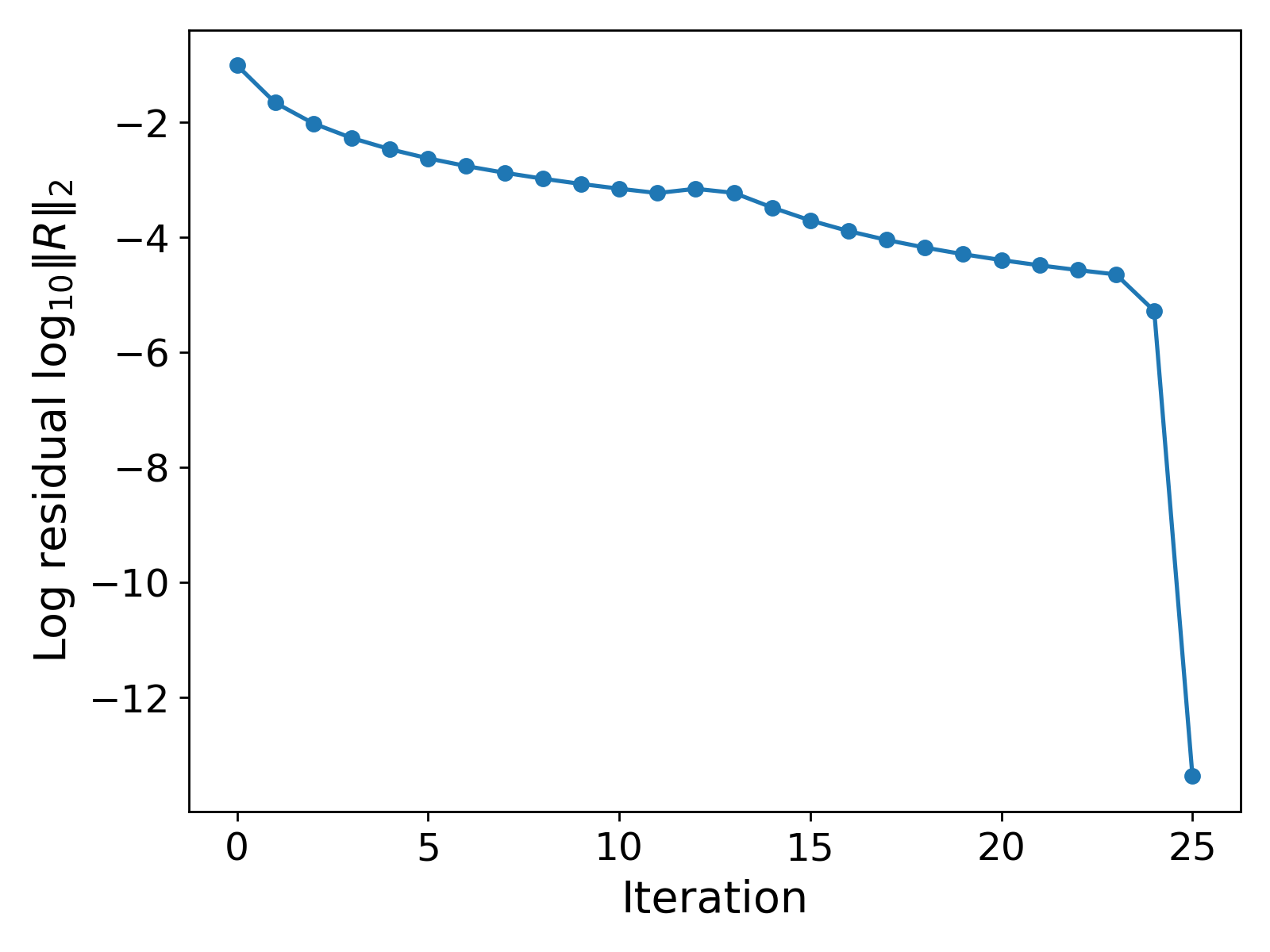
We use $M = 25$ cells, an initial guess of ${u_h}^{(0)} = 0$, and a prescribed tolerance of $\epsilon = 10^{-8}$. The results are shown in Fig. 3.

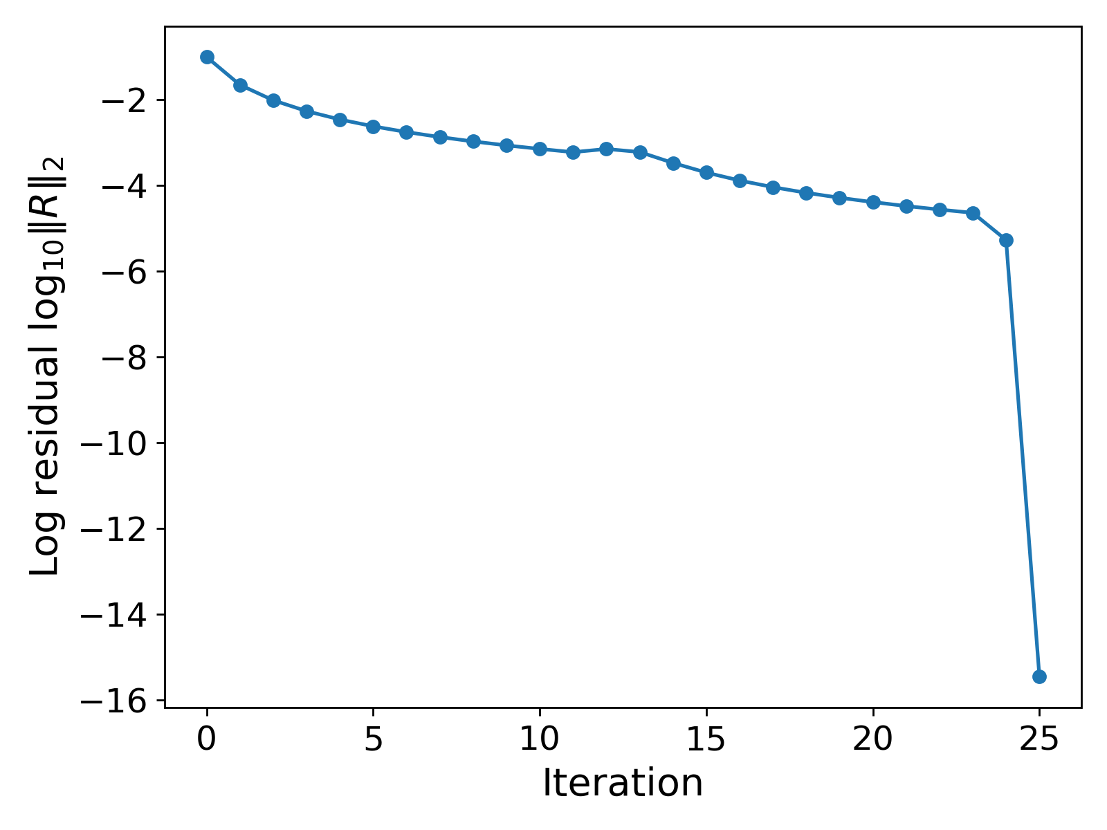
It can be observed that the solution $u_h$ is $0$ everywhere except at $x = 0.48$, where the source function takes the value $2$. Also, the total number of iterations taken by the CG method is $25$.

Robustness testing: changing the initial guess. The results in Fig. 2. show the convergence of the CG method, and in fact, the solver does not struggle to converge. However, to test the robustness of our solver, we provide a different initial guess. We choose ${u_h}^{(0)} = 1$. If our computational method is indeed robust, then we should still hope for convergence to the same solution profile as shown in Fig. 2. regardless of the initial guess (reasonable intial guess!). The results with this new initial guess are shown in Fig. 4.

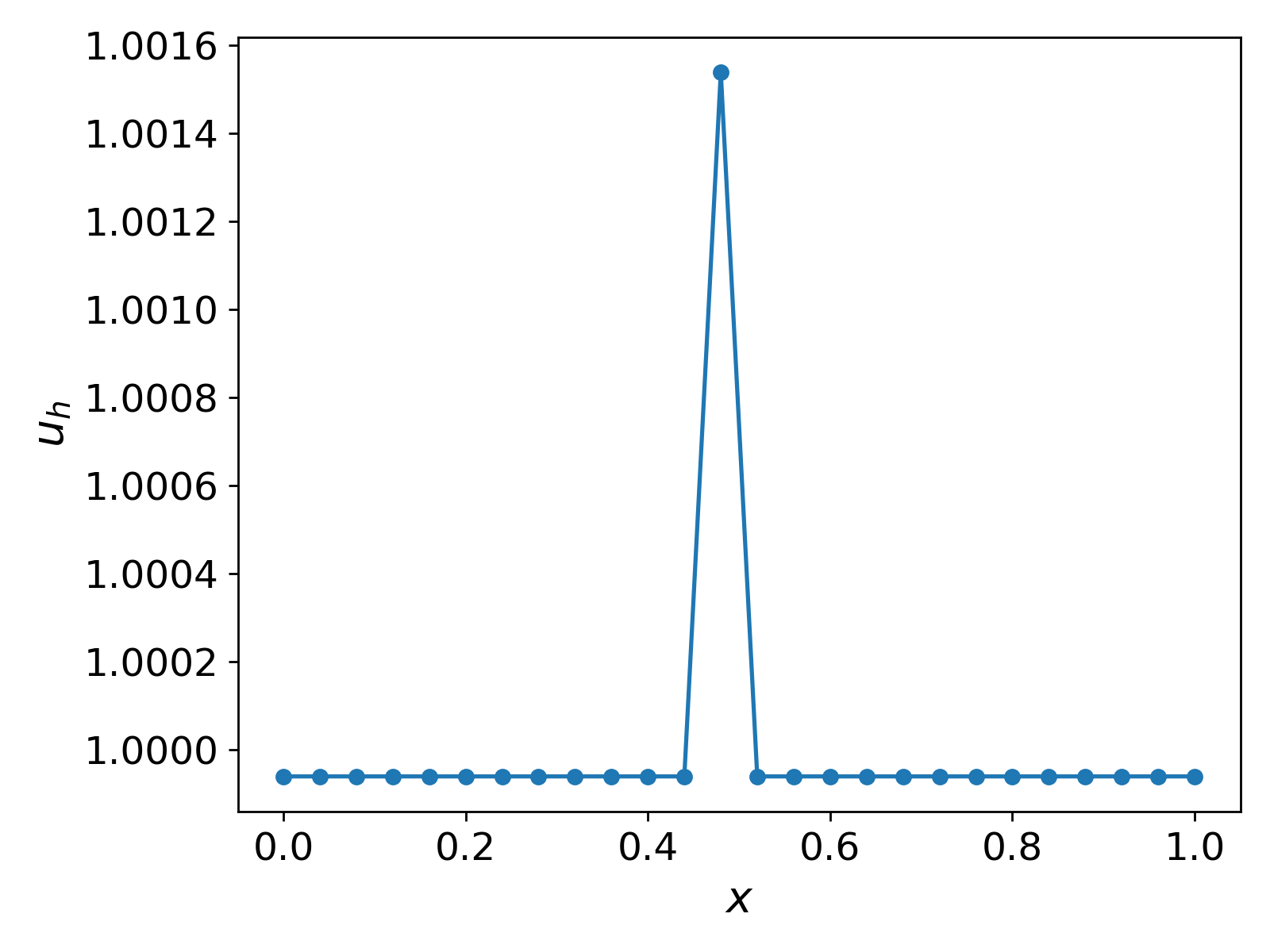
The results in Fig. 3. show a similar profile for $u_h$ as in Fig. 2., but the values differ by $1$! That is, even though we have convergence in both scenarios, the values of the solution are not the same and differ almost by a value of $1$.

The reader may have guessed the reason for this behaviour, and now we make it clear. Even though we have convergence of our CG solver, the problem itself is not well-posed in the first place! That is, the solution to \ref{eq:elliptic_eq} with the given boundary conditions is not unique. It is easy to verify that if $u_h$ solves \ref{eq:variational_form}, then so does $u_h + c$, for any constant $c \in \mathbb{R}$. Thus, for different initial guesses the solver converges to different solutions, which rightfully differ by a constant ($1$ in this case). If one probes further (or already did when setting up the system), it can be verified that the matrix $A$ is singular (and hence not positive definite, but positive semi-definite). Finally, if instead of Neumann boundary equation we would have homogeneous Dirichlet boundary conditions $u(0) = u(1) = 0$, then we would not have run into this issue since the problem would have been well-posed.

This little example highlights the importance of due diligence when it comes to mathematical equations. One may have a convergent solution, but the solution may not make physical sense if prior information regarding the well-posedness of the system is not known. Moreover, in this case, a grid convergence study would have not helped either since for an initial guess the solution would converge to a solution with order $O(h)$.

Note on the choice of quadrature. Note that when computing $\int_{0}^{1} f \phi_j $ in \ref{eq:discretized_system} we make use of the trapezoidal rule. In the example, the function $f$ is non-zero only on a set of measure $0$ and hence the Lebesgue integral $\int_{0}^{1} f \phi_j = 0$. Thus the trapezoidal rule is a poor approximation of this integral. However, we could have obtained the same results as above by using a piecewise-constant $f$ which takes the values $2$ and $-1$ on itervals rather than at points, and for which the trapezoidal rule would have been a better approximation, and we would have obtained the same results as above.

Further Reading and Thoughts

The issue of well-posedness becomes highly nontrivial for coupled multiphysics systems. For example, we may have a system of equations of the form

\begin{equation} \label{eq:multiphysics_coupled} L_1(u, v) = 0, \; L_2(u, v) = 0, \end{equation}

where $L_1, L_2$ are two differential operators. For systems like \ref{eq:multiphysics_coupled} an iterative approach of the form: given ${u_h}^{(m-1)}, {v_h}^{(m-1)}$, first solve for ${u_h}^{(m)}$ and then ${v_h}^{(m)}$ with an algorithm of the form

where ${L_1}_h$ and ${L_2}_h$ are appropriate approximations of $L_1$ and $L_2$, respectively. Such an iterative approach may converge, but it is important do a thorough analysis of the well-posedness of the system beforehand to avoid any spurious non-physical results as explained above.

It is well-known that the CG method converges for non-singular systems; see ^{4 5} for a more thorough analysis.

References

Alexandre Ern, Jean-Luc Guermond, Theory and Practice of Finite Elements, 2004, Springer. ↩ ↩2
Claes Johnson, Numerical solutions of partial differential equations by the finite element method, 1987, Cambridge University Press. ↩
C. T. Kelley, Iterative Methods for Linear and Nonlinear Equations, 1995, Society for Industrial and Applied Mathematics. ↩
Jonathan R Shewchuk, An Introduction to the Conjugate Gradient Method Without the Agonizing Pain, 1994, Carnegie Mellon University. ↩
Hayami, Ken, Convergence of the Conjugate Gradient Method on Singular Systems, 2018, arXiv:1809.00793. ↩