
Investigation into Monotonicity of Solution of the Heat Equation on Fluxes
Date:
1. Introduction
In this post, we investigate the physical impact of oscillations arising due to non-monotone schemes for the heat equation; see our discussion in On the Cause of Spurious Oscillations in Stable Numerical Methods for an in-depth analysis of the cause of oscillations. In particular, we are interested in quantifying the discrepancies in the measurable… We return to the heat equation
\[\partial_t \left( c \theta \right) - \nabla \cdot \left(k \nabla \theta \right) = f, \; \text{ in } \Omega.\]We have already demonstrated in our previous post how implicit Euler Galerkin schemes using $P_1/Q_1$ elements violate the monotonicity condition of the solution, i.e., they do not preserve the positivity of the solution. Physically, we observe negative temperature values in the absence of any sink terms or negative Dirichlet boundary conditions. An in-depth analysis shows how the scheme becomes non-monotone, i.e., it does not preserve the positivity of the solution when the thermal conductivity or time step becomes too small. We also develop a scheme using appropriate quadrature that solves this issue and produces a monotone scheme, thereby eliminating the spurious oscillation causing negative temperature values.
1.1. Example setup
We now explore how much impact these oscillations have on a measurable quantity such as the average temperature over a given subset of one of the boundary faces. To this end, we consider a three-dimensional heterogeneous domain as shown below.
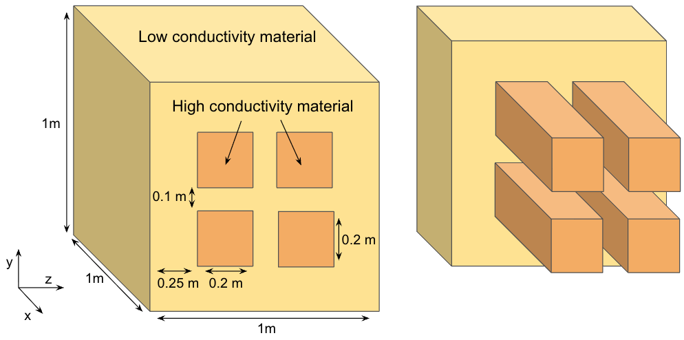
The thermal conductivity and heat capacity for the two types of materials is $k_{high} = 1000$ [J/m $^\circ$ C s], $c_{high} = 10^6$ [J/m$^3$ s] and $k_{low} = 0.01$ [J/m $^\circ$ C s], $c_{low} = 10^6$ [J/m$^3$ s].
2. Numerical Scheme and Solver
We consider first order implicit time stepping and spatial discretization using $Q_1$ bilinear elements. We consider two aproaches: (a) using the full quadrature when computing the mass matrix (Gaussian quadrature) and (b) using the trapezoidal rule to compute the mass matrix; see On the Cause of Spurious Oscillations in Stable Numerical Methods for complete details of the two approaches. We now know that approach (a) will lead to negative temperature values and (b) will preserve the positivity and bounds of the solution.
We develop and implement our scheme in deal.II 1. To efficiently handle the large scale of the problem, we parallelize our implementation using MPI and PETSc 2, the interface of which is offered in deal.II itself. As part of the linear solver, we consider the conjugate gradient (CG) method with the algebraic multigrid (AMG) preconditioner.
2.1. Measured Quantity
In order to compare the two approaches, we compute the temperature average on a subset of one of the boundaries
\[\label{eq:measured_value} \overline{\theta^n} = \frac{\int_{\Omega_M} \theta^n_h }{\int_{\Omega_M} 1},\]where $\theta^n_h$ is the discretized solution obtained at time step $n$, and $\Omega_M \subset \partial \Omega$ is a chosen subset. The motive for chosing \ref{eq:measured_value} is that it allows us to measure the temperature at one face of the heating object thereby mimicing actual physical measurements.