1. Introduction

We start by considering a simple example of heat conduction and temperature change in an object over a time period $(0, T)$. Consider an object with volumetric heat capacity $c$ [J/m$^3$ $^\circ C$]. We add heat to this object at the rate of $f(t)$ [J/m$^3$ s]. Ignoring any spatial variation, the temperature $\theta(t)$ [$^\circ$ C] of the object can be determined using the ODE¹

\begin{equation} \label{eq:heat_eq} \dot{(c \theta)} = f \text{ in } (0, T). \end{equation}

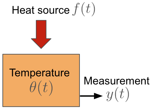
Now, let us measure the temperature using an external sensor, and we denote the measurement using $y(t)$ [$^\circ$ C]; see Fig. 1 below for a schematic. The measurement is represented by

\begin{equation} \label{eq:measurement_heat} y(t) = \theta(t), \; \forall t \in (0, T). \end{equation}

Let us proceed with a discretization of \ref{eq:heat_eq}. Let $\tau$ denote the given time step, and let $N = T/\tau$ be the total time steps. Let $\tilde{f} \approx f, \; \tilde{f} \in C^0(0, T)$ be a piecewise-constant approximation given by

\begin{equation} \label{eq:f_assum} \tilde{f}(t) = f_k = f(k \tau), \; \forall t \in \left(k\tau, (k+1)\tau \right), \; \forall k \in \mathbb{Z}^{+}. \end{equation}

Under the assumption \ref{eq:f_assum}, the solution to

\begin{equation} \label{eq:heat_eq1} \dot{(c \theta)} = \tilde{f} \text{ in } (0, T), \end{equation}

is given by $\theta(t) = \int_0^t c^{-1} \tilde{f}(z)dz \in H^1(0, T)$, which is piecewise-linear. To estimate $\theta$, we can rewrite \ref{eq:heat_eq1} as

\begin{equation} \label{eq:heat_disc} \theta_{k+1} = \theta_k + \tau c^{-1} f_k, \end{equation}

where $\theta_k = \theta(k \tau)$. Now, if we are given $\theta_0 = \theta(0)$, we can compute $\theta_k \; \forall k$. But what about the measurement equation given by \ref{eq:measurement_heat}? We can discretize that trivially as

\begin{equation} \label{eq:measurement_heat_disc} y_k = \theta_k, \end{equation}

where $y_k = y(k \tau)$.

Now, consider the following problem.

Problem statement. Suppose we are given the sequence $y_k, \; 1 \leq k \leq N$ Can we estimate $ \theta_k, \; 1 \leq k \leq N$ using the system \ref{eq:heat_disc}-\ref{eq:measurement_heat_disc}? In other words, at each time step $k$, we seek the “best” estimate $\hat{\theta_k}$ of $\theta_k$ with our knowledge of $ y_j, f_j, \; 1 \leq j \leq k$.

In a perfect world, yes of course, without any error, since in a “perfect” world the temperature of the object changes “perfectly” according to \ref{eq:heat_disc} without any erro which gives us $\theta_k = y_k$ exactly. However, in reality, we expect some noise to be introduced when the temperature changes which can be represented as

\begin{equation} \label{eq:heat_disc1} \theta_{k+1} = \theta_k + \tau c^{-1} f_k + w_k, \end{equation}

where $w_k$ is the process noise. Morever, in a world of noisy sensors and less perfect measuring equipments, we can also assume that some error is introduced in the measurements $y_k$, i.e., instead of \ref{eq:measurement_heat_disc}, we have an equation similar to

\begin{equation} \label{eq:measurement_disc1} y_k = \theta_k + v_k, \end{equation}

where $v_k$ is the measurement noise. Before we exemplify the problem, we first establish some notation. We call $\theta_k$ in \ref{eq:heat_eq} the true state of the temperature.

1.1 Example

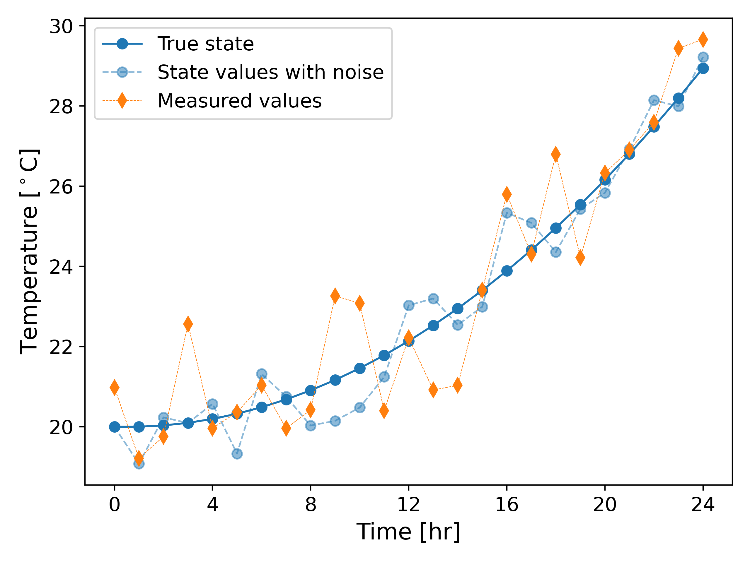
As an example, we consider the heating of the object over the time period $(0, 24)$ [hr]. We consider $c = 10^6$[J/m$^3$ $^\circ$ C] and $f(t) = 0.0025 t$ [J / m$^3$ s]. Fig. 2 below shows the true temperature, the temperature evolution according to \ref{eq:heat_disc1}, and the measured temperature values. Here we assume that $v_k$ and $w_k$ are uncorrelated Gaussian random processes with zero mean and standard deviation $\sigma_w = 0.75$ and $\sigma_v = 1.25$, respectively.

The problem statement now becomes nontrivial: given $y_k, \; 1 \leq k \leq N$ how can we accurately estimate $\theta_k, \; 1\leq k \leq N$ using \ref{eq:measurement_disc1}-\ref{eq:heat_disc1}? In other words, how do we compute the best estimate $\hat{\theta_k}$ that approximates $\theta_k \; \forall 1 \leq k \leq N$?

2. Kalman filter

We now present the Kalman filtering technique. Consider a simple 1D linear state-space system of the form

\begin{equation} \label{eq_state} \dot{x(t)} = A x(t) + B u(t), \end{equation}

\begin{equation} \label{eq_output} y(t) = C x(t) + D u (t), \; \forall t \in (0, T), \end{equation}

where $x \in \mathbb{R}$ is the state variable, $u \in \mathbb{R}$ is the input, $y \in \mathbb{R}$ is the output, $A, B, C, D \in \mathbb{R}$ are constants. We assume $u$ to be a piecewise-constant as in \ref{eq:f_assum}. Then, a simple integration by parts yields²

\begin{equation} \label{eq_disc_state} x_{k+1} = e^{A \tau} x_k + \left(\int_{0}^{k\tau} e^{A z} dz \right) B u_k, \end{equation}

\begin{equation} \label{eq_disc_output} y_k = C x_k + D u_k, \end{equation}

where $\tau$ is the time step, and $x_k = x(\tau k)$ is the value at the $k^{th}$ time step (in this case the exact value of the continuous solution!), with similar definition for $y_k$. Note that \ref{eq_disc_state} does not introduce any truncation error due to time discretization.

Algorithm. The Kalman filter is a recursive algorithm that first predicts $\hat{x_k}^{-}$ using the state equation and then uses the measurement $y_k$ to further correct $\hat{x_k}^{-}$ and produce a more accurate $\hat{x_k} \approx x_k$. Let $\hat{e_k}^- = \hat{x_k}^- - x_k$ and $\hat{e_k} = \hat{x_k} - x_k$ denote the corresponding errors, and $\hat{\Sigma_k} = \mathbb{E}[\hat{e_k}^2], \; \hat{\Sigma_k}^- = \mathbb{E}[{\hat{e_k}^-}^2]$ be the covariances. The algorithm is follows³.

1. Initialization. Let $\hat{x_0} = x_0$ and $\hat{\Sigma_0} = 0$.

2. Prediction step (a priori estimate). Given $\hat{x_{k-1}}$, we compute $\hat{x_k}^{-}$ and $\hat{\Sigma_k}^{-}$ using

\begin{equation} \hat{x_k}^{-} = A \hat{x_{k-1}} + B u_{k-1} \end{equation}

\begin{equation} \hat{\Sigma_k}^{-} = A^2 \hat{\Sigma_{k-1}} + \Sigma_w \end{equation}

3. Correction step (a posteriori estimate). In this step, we first compute the Kalman gain, $L_k$, as follows

\begin{equation} L_k = \hat{\Sigma_k}^- C \left(C^2 \hat{\Sigma_k}^- + \Sigma_v \right)^{-1}. \end{equation}

Then, we compute $\hat{x_k}$ and $\hat{\Sigma_k}$ using

\begin{equation} \hat{x_k} = \hat{x_k}^- + L_k \left(y_k - C \hat{x_k}^{-} - D u_k \right), \end{equation} \begin{equation} \hat{\Sigma_k} = \left(I - L_k C\right) \hat{\Sigma_k}^-. \end{equation}

2.1 Example: Heat Equation

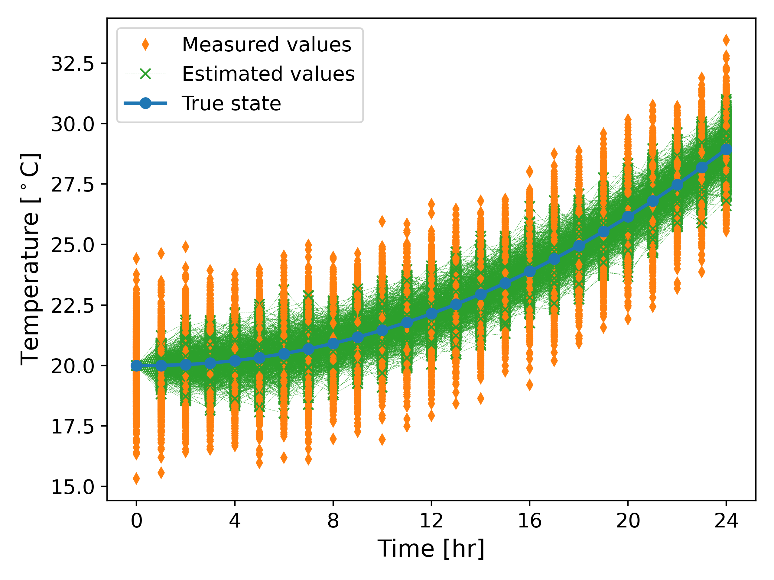
We now return to our example. We consider an intial condition $\hat{\theta_0} = y_0$ and $\hat{\Sigma_0} = 0$, and run the Kalman filter. The results are shown in Fig. 3.

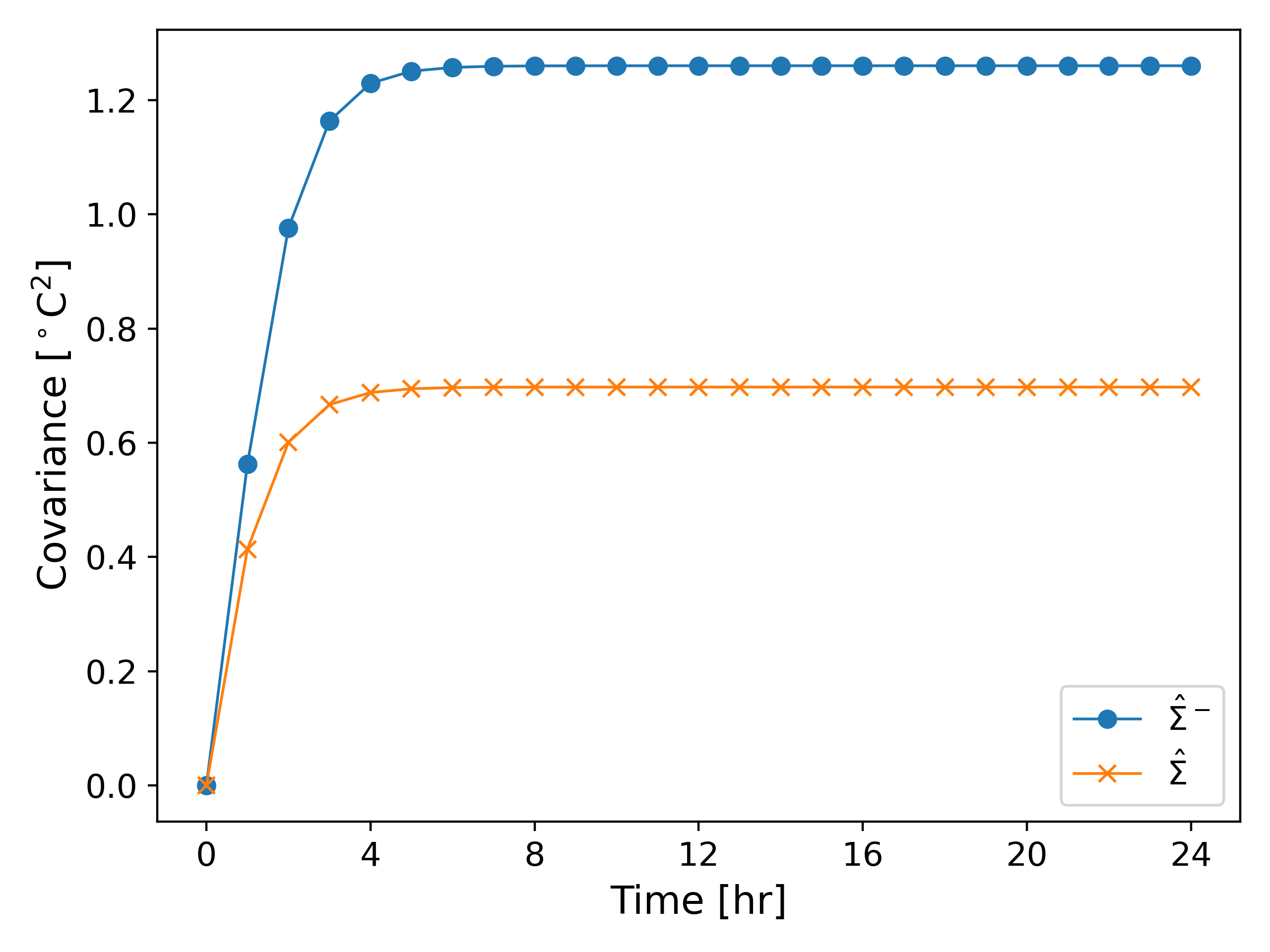
It can be observed from Fig. 3 that the estimated temperature is much more aligned to the true state than the measured values. Fig. 3 also shows the predicted and estimated covariance and it can be observed that the corrected covariance is always lower than the predicted covariance, although both values quickly reach a steady state.

2.2 Variance Estimation: Monte Carlo Simulations

We also compute the variance of the estimated values ($\hat{\theta}$) and the measured values ($y$) denoted by $\sigma_{\hat{\theta}}^2$ and $\sigma_y^2$, respectively. We run $1000$ simulations using the same random parameters as earlier; see Fig. 5 below.

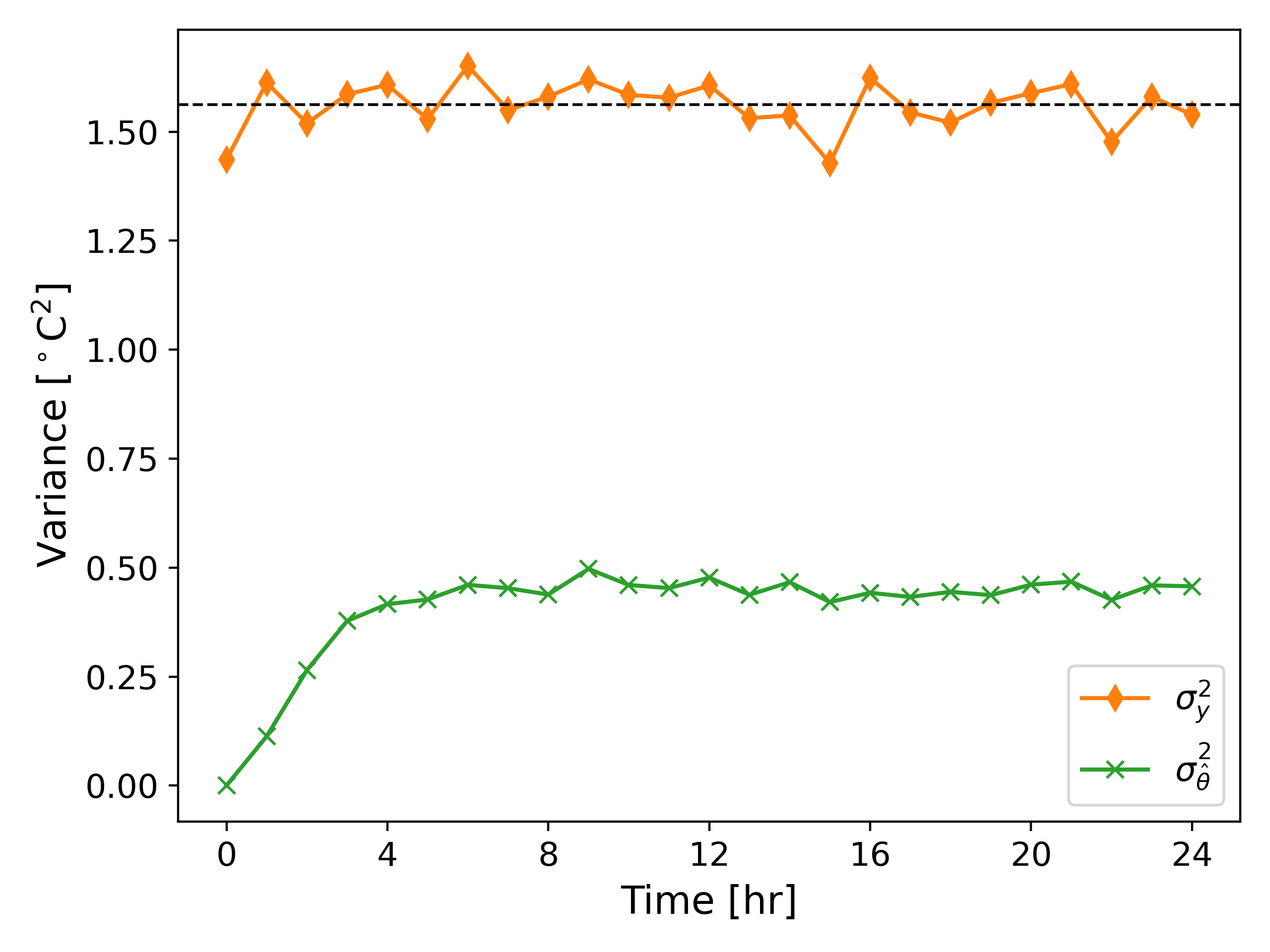
It can be observed from Fig. 6 that the variance of the estimated values is much smaller than the variance of the measured values, and even smaller than the variance of the process noise $\approx 0.562$. This exercise demonstrates the effectiveness of the Kalman filter in reducing the error between the measured values and the true state.

Further Reading

The discussion above presents a basic introduction to the use of Kalman filters for optimal filtering. We demonstrate the use of the Kalman filter in 1D, although the implementation can easily be extended to higher dimensions³. A brief introduction to the algorithm can also be found in an article by Welch, Bishop, 2006⁴.

References

H.S. Carslaw, J. C. Jaeger, Condution of Heat in Solids, 1959, Oxford University Press. ↩
Chi-Tsong Chen, Linear System Theory and Design, 1999, Oxford University Press, 3rd Edition. ↩
Gregory L. Plett, Extended Kalman filtering for battery management systems of LiPB-based HEV battery packs, Part 1, Background, 2004, Journal of Power Sources. ↩ ↩2
Greg Welch, Gary Bishop, An Introduction to Kalman Filter, 2006 (available online). ↩