1. Introduction

In this post, we investigate two approaches to solving the heat equation on $\Omega \subset \mathbb{R}^3$

where $\theta$ [$^\circ$ C] is the temperature, $c$ [J/m$^3$ $^\circ$ C] is the known volumetric heat capacity of the material, and $k = k(x)$ [J/m $^\circ$ C s] is the known thermal conductivity. We are interested in quantifying the discrepancies in measurable quantities, such as the average temperature over a subset of the boundary face.

We consider (a) non-monotone implicit and (b) monotone implicit scheme. We wish to quantify the differences in these two approaches when simulating a physical scenario of an object heating. In our previous post, we investigated the cause of spurious numerical oscillations arising due to a non-monotone scheme (in cases of low time step size and low thermal conductivity); see our discussion in On the Cause of Spurious Oscillations in Stable Numerical Methods for an in-depth analysis of the cause of oscillations.

We have already demonstrated in our previous post how implicit Euler Galerkin schemes using $P_1/Q_1$ elements violate the monotonicity condition of the solution, i.e., they do not preserve the positivity of the solution (and the initial bounds). Physically, we observe negative temperature values in the absence of any sink terms or negative Dirichlet boundary conditions. An in-depth analysis shows how the scheme becomes non-monotone, i.e., it does not preserve the positivity of the solution when the thermal conductivity or time step becomes too small. We also developed a scheme using appropriate quadrature that solves this issue and produces a monotone scheme, thereby eliminating the spurious oscillation causing negative temperature values. However, the monotone scheme introduces quadrature error since we use the trapezoidal rule, as opposed to the Gaussian quadrature which is exact for polynomials. Hence, we expect some inaccuracy to arise because of this approach as well.

Thus the question we seek to answer is this: is the quadrature error worth helping us remove non-physical oscillations insofar as the accuracy of the scheme is concerened?. Although there are numerous higher accuracy monotone schemes in literature, here we are concerned with the one that we have obtained previously, i.e., a first order implicit time stepping scheme using Q1 elements.

We now explain the heterogeneous physical scenario used in our investigation.

1.1. Example Setup

We now simulate a physical scenario to understand the effect of the negative temperature oscillations produced by the Gaussian quadrature compared to the inconsistency introduced by the trapezoidal quadrature. To this end, we consider a three-dimensional heterogeneous material occupying $\Omega = (0,1)^3$ [m$^3$] as shown below.

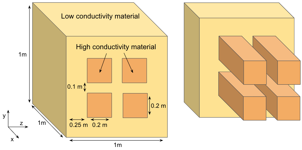
The thermal conductivity and heat capacity for the high conductivity material is $k = 1000$ [J/m $^\circ$ C s], $c = 10^6$ [J/m$^3$ s] and for the low conductivity material is $k = 0.20$ [J/m $^\circ$ C s], $c = 10^7$ [J/m$^3$ s]. We consider Dirichlet boundary conditions on $\{ 0 \} \times (0,1) \times (0,1)$ where we set $\theta = 1$ [$^\circ$ C], and on the other faces we consider the Neumann no-flux boundary condition $\nabla \theta \cdot \nu = 0$.

1.2. Measured Quantity: Average Temperature

In order to compare the approaches (a) and (b), we compute the temperature average on a subset of one of the boundaries

where $\theta^n_h$ is the discretized solution obtained at time step $n$, and $\Gamma_F \subset \partial \Omega$ is a chosen subset. The motive for chosing \ref{eq:measured_value} is that it allows us to measure the temperature at one face of the heating object thereby mimicing actual physical measurements.

For our numerical results, we consider $\Gamma_F = \{ 1 \} \times (0.25, 0.75) \times (0.25, 0.75)$.

1.3. Reference Solution

Since for the above example we do not have an analytical solution, we compute the reference solution on a fine grid (low spatial grid size and time step) to help us quantify the differences in our approaches when computing the average temperature \ref{eq:measured_value}. In order to do this efficiently, we implement our solver in parallel; see the next section for details.

2. Numerical Scheme and Solver

We consider first order implicit time stepping and spatial discretization using $Q_1$ bilinear elements. We consider two aproaches: (a) using the full quadrature when computing the mass matrix (Gaussian quadrature) and (b) using the trapezoidal rule to compute the mass matrix; see On the Cause of Spurious Oscillations in Stable Numerical Methods for complete details of the two approaches. We now know that approach (a) will lead to negative temperature values and (b) will preserve the positivity and bounds of the solution.

We develop and implement our scheme in deal.II ¹. To efficiently handle the large scale of the problem, we parallelize our implementation using MPI and PETSc ², the interface of which is offered in deal.II itself. As part of the linear solver, we consider the conjugate gradient (CG) method with the algebraic multigrid (AMG) preconditioner.

3. Results

To compare our approaches (a) and (b), we first compute the reference solution using a really fine spatial mesh. We run the simulation over $(0, 24)$ [hr] using a time step of $\tau = 0.25$ [hr], and a uniform spatial mesh using edge length $0.00625$ [m] (corresponding to more than 4 million degrees of freedom!). The simulation is launched on 10 processors, and the results at the a few time steps are shown in Fig. 2. The simulations takes roughly 3.8 hours to finish on my pesonal macbook, with maximum 13 iterations for the CG solver per time step.

Owing to the highly heterogeneous nature of the example, most of the temperature change happens in the high conductivity region represented by the 4 rectangular bars (as shown in the sliced view in Fig. 2.). The other part of the domain does not show much temperature variation, and by $12$ [hr] the solution almost appears to reach a steady state value.

We now compute the solution using the Gaussian quadrature and trapezoidal quadrature on a uniform mesh with cell width $h = 0.05$ [m], and compute the average temperature given by \ref{eq:measured_value}, and we use a time step $\tau = 2.0$ [hr]. At this discretization scale, negative temperature values were observed in approach (a). The average temperature is shown in Fig. 3.

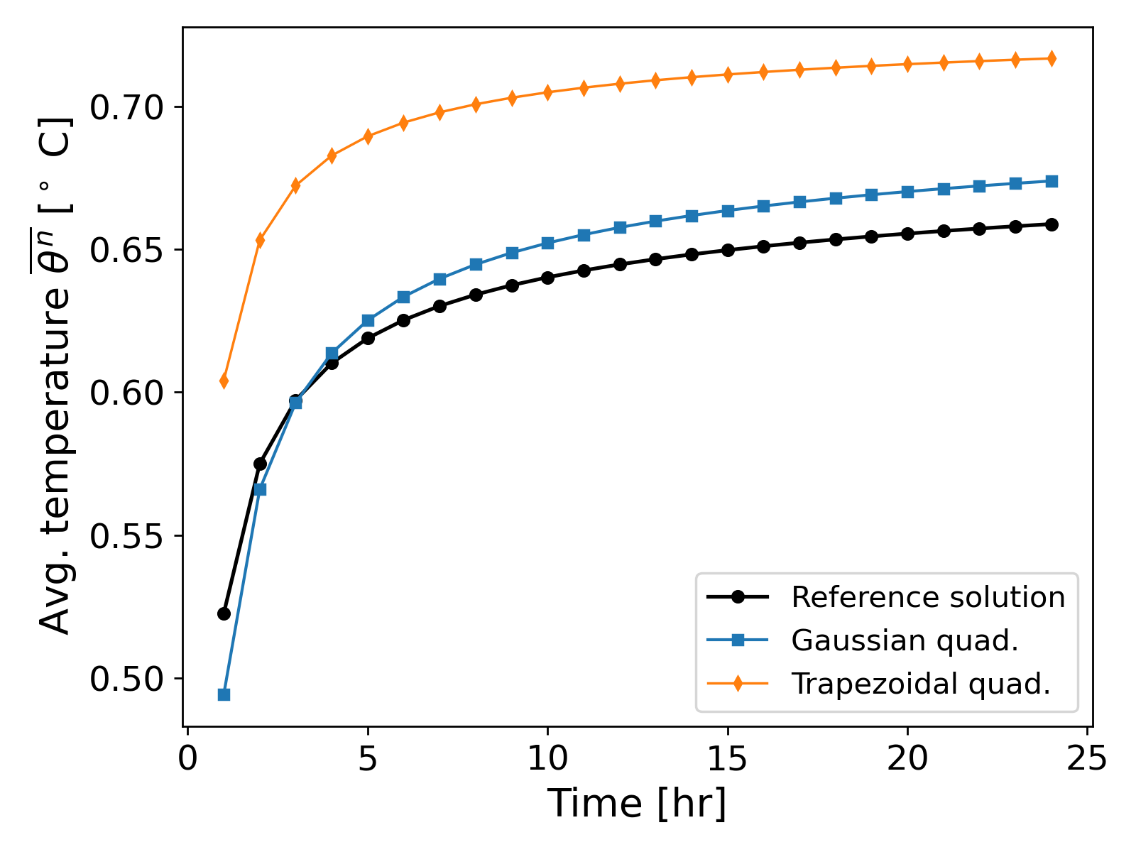
The temperature error over the entire simulation time period for approach (a) is $\lVert \overline{\theta^n} - \overline{\theta^n_{ref}} \rVert_\infty = 0.1590$ [$^\circ$ C] and for approach (b) $\lVert \overline{\theta^n} - \overline{\theta_{ref}^n} \rVert_\infty = 0.2323$ [$^\circ$ C], where $\theta^n_{ref}$ referes to the reference solution at time step $n$. The error shows a significant difference between the two approaches.

Discussion of results. It can be observed from Fig. 3. that the Gaussian quadrature (approach (a)) yields values closer to the reference solution than the trapezoidal quadature (approach (b)) when using a coarse mesh, even though spurious oscillations (negative temperature values) are present when using the Gaussian quadrature. That is, even though the trapezoidal quadrature leads to positivity preserving scheme, the error introduced by the quadrature itself leads to large differences in the measured average temperature values.

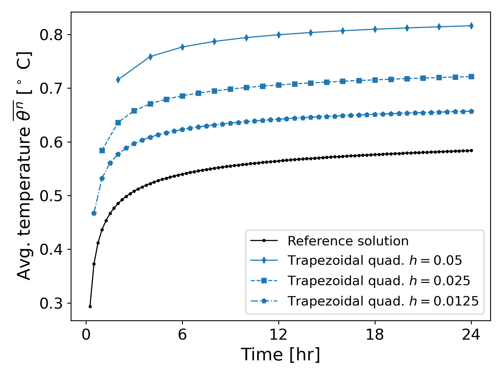
At first glance, it might seem questionable if approach (b) even converges to the reference solution. However, a quick grid convergence study where we refine the cell width edge to be $h \in \{0.05, 0.025, 0.0125\}$ [m] with corresponding $\tau \in \{2, 1, 0.5 \}$ [hr] shows that the average temperature values actually approach the reference solution; see Fig. 4.

On the solver side, not much of a difference exists between the two approaches. The CG iterations for both approaches are about 12-13 per time step (with the AMG preconditioner).

Summary. The above example demonstrates that even in the presence of spurious oscillations, approach (a) yields results closer to the reference solution when computing the average temperature. However, approach (b) is not without its merits: at very small time steps (even for a fine grid), spurious oscillations from approach (a) tend to dominate the soundness of the physical problem (i.e. how can we have negative temperatures in a heating scenario?) and approach (b) would yield more physically sound results, since a smaller grid size also means that the quadrature error decreases.

Further Reading

The above example demonstrated the seemingly negligible effect of spurious oscillations on average measured temperature. While in this case, it appears that using the conditionally monotone approach (a) is more accurate, care must be taken in multiphysics problems. That is, suppose we were to reconstruct a continuous flux $\tilde{q} \approx -k \nabla \theta$, and use it in coupled transport problem of the form

where $C$ measures some concentration. Then how would these spurious oscillations transfer over to the numerical solution of \ref{eq:coupled_problem_transport}? The author of this blog has already demonstrated the presence of similar oscillations in mixed finite elements ³, when the full quadrature is used to compute the mass matrix of H$_{div}$ Raviart-Thomas elements. It would be an interesting idea to explore how monotone schemes interact with each other in multiphysics problems, although that is the subject of a future blog post.

References

Daniel Arndt et al., The deal.II library, Version 9.7, Journal of Numerical Mathematics, 2025. ↩
S. Balay et al., PETSc/TAO Users Manual ANL-21/39 - Revision 3.24, OSTI.GOV, 2025. ↩
Vohra, N. and Peszynska, M., Robust conservative scheme and nonlinear solver for phase transitions in heterogeneous permafrost, 2024, Journal of Computational and Applied Mathematics. ↩