1. Introduction

Neural Networks may have been around since the 1940s^{1 2}, but their importance and popularity has permeated the current era. Although a lot of articles and web pages talk about their applications, here we discuss the building blocks of neural networks. In particular, we are interested in their mathematical framework, and how they can be used in interpolation and forecasting.

1.1. Components of a Neural Network

A neural network may be viewed as a black-box solver that can be “trained” to take an input $t$ and returns an output $y$. For example, suppose we have measured the outside temperature at every hour during the day, but are interested in finding the temperature at $1:45$PM, or around noon the next day. A solution to this is to train a neural network on the hourly temperature values that have been measured to predict the value at any time (down to seconds, minutes etc.).

A simple architecture of a neural network similar to that shown in Fig. 1. Here we consider a network that takes $t \in \mathbb{R}$ as an input and gives $y \in \mathbb{R}$ as an output. The hidden layer consists of weights and biases $w_{1,i}, b_{1,i}, w_{2,i} \in \mathbb{R}, \; 1 \leq i \leq 5$, and $b_2 \in \mathbb{R}$, along with a nonlinear smooth activation function $\sigma : \mathbb{R} \rightarrow \mathbb{R}$.

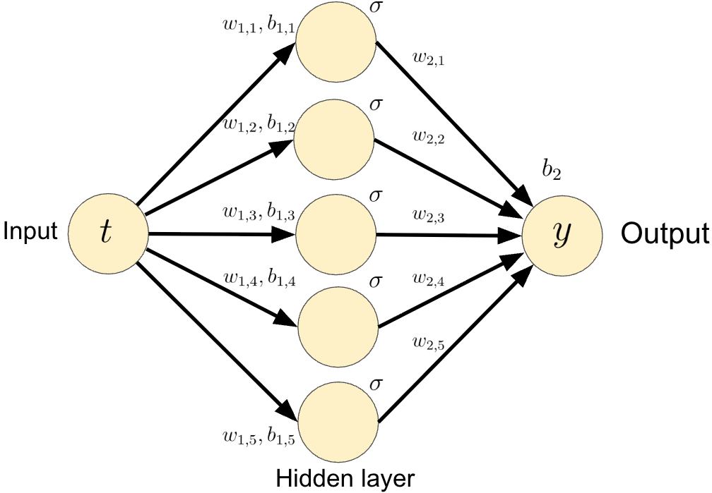
In this case, the output $y$ is given by

\begin{equation} \label{eq:nn_ex1} y = \sum_{i=1}^{5} \sigma\left( w_{2,i} \sigma\left(t w_{1,j} + b_{1,i} \right) + b_{2} \right). \end{equation}

Or, more succinctly, using matrix vector notation, we rewrite \ref{eq:nn_ex1} as

\begin{equation} \label{eq:nn_ex2} y = \sigma \left( {w_2}^T \sigma \left(w_1 t + b_1 \right) + b_2 \right) \end{equation}

where $w_1 = [w_{1,1} \; w_{1,2} \; w_{1,3} \; w_{1,4} \; w_{1,5} ]^T$ (similar definition for $b_1$ and $w_2$), and $\sigma$ is applied component wise to the vector $w_1 x + b_1$.

Now let us assume that we are given $N \in \mathbb{Z}$ measurements of $y$, denoted by $\hat{y}_n, \; 1 \leq n \leq N$ for corresponding inputs (known) $t_n$. Consider the following problem statement.

Problem statement. How do we find the parameters $w_1, b_1, w_2$ and $b_2$ such that each $y_n$ obtained using $x_n$ from \ref{eq:nn_ex1} is `sufficiently close’ to $\hat{y}_n$?

1.2. Minimizing the Loss

In order to select the appropriate parameters $\mathbf{w} = [{w_1}^T \; {b_1}^T \; {w_2}^T \; {b_2}]^T$ we provide a number to what `sufficiently close’ means. To this end, we specify the mean squared error (MSE) as

\begin{equation} \label{eq:loss_function} E = \frac{1}{N}\sum_{n=1}^{N} E_n, \; E_n = \left(\hat{y}_n - y_n \right)^2. \end{equation}

We now seek to find the best parameters that minimize the loss function $E$ given by \ref{eq:loss_function}. One of the most popular techniques is the gradient descent algorithm: let $\eta > 0$ be given. Define an iterative process as follows: given $\mathbf{w}^{(j)}$, perform the update

\begin{equation} \label{eq:gradient_descent} \mathbf{w}^{(j+1)} = \mathbf{w}^{(j)} - \alpha \nabla_{\mathbf{w}} E\left(\mathbf{w}^{(j)}\right), \end{equation}

where $\nabla_{\mathbf{w}} E = \left[ \nabla_{b_1}^T E \; \nabla_{w_1}^T E \; \nabla_{w_2}^T E \; \partial_{b_2} E \right]^T$ denotes the Jacobian of $E$ with respect to $\mathbf{w}$. Under a suitable $\eta > 0$ and initial guess $\mathbf{w}^{(0)}$, the sequence $\{w^{(j)}\}$ generated by \ref{eq:gradient_descent} converges to the minimizer of $E$. The parameter $\eta$ is known as the learning rate and is specified apriori.

1.3. Error Backpropagation

Backpropagation is a popular concept which denotes the passing of the information “backward” through the network. In essence, when computing the gradient $\nabla_{\mathbf{w}} E$, owing to the smooth nature of all the functions, the chain rule can be effectively utilized which prevents computing the derivatives again and again through multiple hidden layers². We do not explore that in any detail here, since that is out of scope of the aim of this post.

We are now ready to implement our first neural network. We make use of the popular Python library NumPy³.

2. Example: Approximating a Cosine Wave

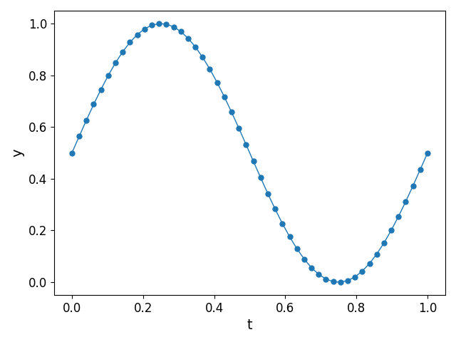
We consider the measurements of a cosine wave $y = \cos{(2\pi t)}$ at $N = 50$ regularly spaced points $t_n$ as shown in Fig. 2.

2.1. Implementation Details

We use the activation function $\sigma(x) = \tanh{(x)}$. Since the data already lies in the range of the activation function, we do not scale the data any further (say so that it lies in [-1,1]). We also train the network for a maximum of $10000$ iterations, which we refer to as `epochs’, and consider a learning rate of $\eta = 0.01$ (concluded from a heuristic approach). Finally, we initialize the parameters $\mathbf{w}^{(0)}$ using a Normal distribution $N(0,1)$.

2.2. Results

We plot the output of the network at different epochs in Fig. 3. It can easily be observed that the approximation \ref{eq:nn_ex2} `approaches’ the measured values as the epochs increase (in the eyeball norm!).

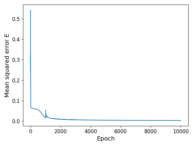
The final trained network at the end of $10000$ epochs, along with a plot of the MSE vs the epochs is shown in Fig. 4. It can be observed that the MSE decreases and plateaus towards the end as the parameters converge.

3. Moving Forward

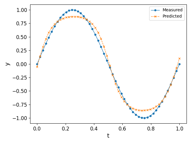
The above discussion shows how effectively a basic neural network may approximate given data, insofar as interpolation is concerned. However, when it comes to extrapolating (or predicting), the above algorithm does not perform well; see Fig. 5 (left) for an illustration when we feed $t > 1$ as an input to the trained network. It can be seen that the neural network does not predict accurate values for $t > 1$, for the simple reason that it does not learn the periodicity of the data. One way to solve this issue is by considering an activation function that has an inherent periodicity⁴.

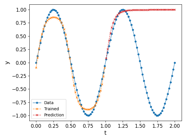
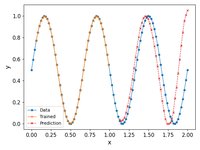
In the next post, we show how we can circumvent this problem to some degree using Recusrive Neural Networks (RNN), and by rearranging the input dataset to conform with supervised learning techniques. We exemplify this in Fig. 5 (right): indeed, it can be observed that the predicted values are much closer to the periodic nature of the data as opposed to the simple network constructed in this post.

Code

The code used in this post has been written by the author and can be found below. The user may keep in mind that the point of the code is clarity in exposition, and not super efficiency.

# One layer neural network training.
# Author: Naren Vohra
# Email: NarenVohra1994@gmail.com

import numpy as np
import matplotlib.pyplot as plt

# ################################
# Function definitions
# ################################

# Define function to approximate and interpolate
def my_func(x):
    return np.sin(2 * np.pi * x)

# Define activation function
def sigma(x):
    return np.tanh(x)

def dsigma(x):
    return (1 - np.tanh(x)**2)

# Initialize weights and biases
def intialize_weights(n_size):
    # Set random seed for reproducibility
    np.random.seed(42)
    w1 = np.random.normal(loc = 0.0, scale = 1.0, size = (n_size, 1))
    w2 = np.random.normal(loc = 0.0, scale = 1.0, size = (n_size, 1))
    b1 = np.random.normal(loc = 0.0, scale = 1.0, size = (n_size, 1))
    b2 = np.random.normal(loc = 0.0, scale = 1.0, size = (1, 1))

    return w1, w2, b1, b2

# Feed forward first stage: z = \sigma(w1 x + b1)
def feed_forward1(x, w1, b1):
    z = sigma(w1 * x + b1)
    return z

# Feed forward second stage: \sigma(w2 z + b2)
def feed_forward2(z, w2, b2):
    y_hat = sigma(np.dot(w2.T, z) + b2)
    return y_hat

# Compute gradients
def gradients(x, w1, b1, w2, b2):
    z = feed_forward1(x, w1, b1)

    # Calculate gradients
    dEdw1 = dsigma(np.dot(w2.T, z) + b2) * w2 * dsigma(w1 * x +  b1) * x
    dEdb1 = dsigma(np.dot(w2.T, z) + b2) * w2 * dsigma(w1 * x +  b1)

    dEdw2 = dsigma(np.dot(w2.T, z) + b2) * z
    dEdb2 = dsigma(np.dot(w2.T, z) + b2)

    return dEdw1, dEdb1, dEdw2, dEdb2

# Loss function (MSE)
def loss_fn(y, y_hat):
    square_vals = np.abs(y - y_hat) ** 2
    return square_vals.sum() / (2.0 * len(y))

# ################################
# Main script
# ################################

# Create dataset
x = np.linspace(0, 1.0, 50)
x = x.reshape(-1,1)
y = my_func(x)

# Specify size of network and other parameters
n_size = 5
n_epochs = 10000
eta = 0.01

# Initialize weights
w1, w2, b1, b2= intialize_weights(n_size)
print("Parameters initialized")

# Initialize list to store MSE values
loss_list = []

# Start training network
for epoch in np.arange(0, n_epochs, 1):

    # Initialize gradients for each time step
    dEdw1_sum, dEdb1_sum, dEdw2_sum, dEdb2_sum = 0, 0, 0, 0

    # Initalize predicted value
    y_hat = 0.0 * x

    for j in np.arange(0, len(x), 1):
        # Get y_hat
        z = feed_forward1(x[j], w1, b1)
        y_hat[j] = feed_forward2(z, w2, b2)

        # Calculate gradients 
        dEdw1, dEdb1, dEdw2, dEdb2 = gradients(x[j], w1, b1, w2, b2)

        # Add gradients to final vector
        dEdw1_sum += dEdw1 * (y_hat[j] - y[j])
        dEdb1_sum += dEdb1 * (y_hat[j] - y[j])
        dEdw2_sum += dEdw2 * (y_hat[j] - y[j])
        dEdb2_sum += dEdb2 * (y_hat[j] - y[j])

    # Compute MSE
    loss = loss_fn(y_hat, y) 
    loss_list.append(loss)

    if epoch % 1000 == 0:
        print(f"MSE loss at epoch {epoch} is {loss}")

    if np.abs(loss) < 1e-4:
        break 

    # Update weights
    w1 = w1 - eta * dEdw1_sum
    b1 = b1 - eta * dEdb1_sum
    w2 = w2 - eta * dEdw2_sum
    b2 = b2 - eta * dEdb2_sum

# Training finished
print(f"Training finished; final MSE = {loss}")
# Final plot of network output
fig = plt.figure()
plt.plot(x, y, linestyle = "-", linewidth = 1, marker = "o", markersize = 4, label = "Measured")
plt.plot(x, y_hat, linewidth = 1.0, linestyle = "--", marker = "x", markersize = 5, label = "Predicted")

plt.xticks(fontsize = 12)
plt.yticks(fontsize = 12)

plt.xlabel("t", fontsize = 14)
plt.ylabel("y", fontsize = 14)

plt.tight_layout()

# Plot MSE
# Convert list to numpy array
loss_np = np.array(loss_list)

# Plot
fig = plt.figure()

plt.plot(np.arange(0, len(loss_np), 1), loss_np, linewidth = 1.5)

plt.xticks(fontsize = 12)
plt.yticks(fontsize = 12)

plt.xlabel("Epoch", fontsize = 14)
plt.ylabel("Mean squared error E", fontsize = 14)

plt.tight_layout()
plt.show()

References

Last updated: March 2026.
Christopher M. Bishop, Pattern Recognition and Machine Learning, 2006, Springer. ↩
Simon Haykin, Neural Networks and Learning Machines, 2009, 3rd edition, Pearson. ↩ ↩2
Liu Ziyin, Tilman Hartwig, Masahito Ueda, Neural Networks Fail to Learn Periodic Functions and How to Fix It, 2020, arXiv e-prints. ↩
Charles R. Harris et al., Array programming with NumPy, 2020, Springer Science and Business Media (LLC). ↩