1. Introduction to Newton’s Method

Newton’s method is a perpetual workhorse that has proven to be one of the most successful and versatile nonlinear solvers. The framework has been applied to cover a large range of nonlinearities, from smooth to semismooth functions. In this post, we present the application of the Newton’s method in solving the Butler-Volmer equation, commonly used in modelling interface conditions in electrochemical domains. We prove the convergence and demonstrate the robustness of the method using physical parameters, and exemplify how convergence may be further accelerated in extreme cases using the primary variable switching technique.

1.1 Algorithm

Let $F \in C^\infty(\mathbb{R}), \; F : \mathbb{R} \rightarrow \mathbb{R}$ be a given smooth function, and we wish to solve $F(x) = 0$. The Newton’s method generates a sequence $\{ x^{(m)} \}$ iteratively: given $x^{(m-1)}$, we obtain $x^{(m)}$ as

\begin{equation} \label{eq:Newton_method1} R^{(m-1)} = F \left(x^{(m-1)} \right), \end{equation}

\begin{equation} \label{eq:Newton_method2} \delta^{(m-1)} = - {J^{(m-1)}}^{-1} R^{(m-1)}, \end{equation}

\begin{equation} \label{eq:Newton_method3} x^{(m)} = x^{(m-1)} + \delta^{(m-1)}, \end{equation}

where $J^{(m-1)} = F’\left( x^{(m-1)} \right)$ is the Frechet derivative (the Jacobian of $F$), and $x^{(0)} = x_0$ is the inital guess which we are given. We iterate till a prescribed tolerance $\epsilon_{tol} > 0$ is reached by the absolute of the residual $R^{(m)}$.

Note on the choice of Jacobian. In the semismooth framework, the Jacobian $J \in \partial_B F(x)$ is the Clarke’s generalized Jacobian which is computed using the B-subdifferential

\begin{equation} \partial_B F(x) = \{ J_F \in \mathbb{R} \; | \; \exists {x_k} \in D_F, \; x_k \rightarrow x, \; \left(F \right)’(x_k) \rightarrow J_F \}, \end{equation}

where for each $x \in D_F \subset \mathbb{R}$, the Fre´chet derivative $F’(x)$ exists ¹.

1.2 Convergence of Newton’s Method

Under the assumptions that $F$ is Lipschitz with a bounded derivative, convergence of the algorithm \ref{eq:Newton_method1}-\ref{eq:Newton_method3} has been established for an appropriate initial guess $x^{(0)}$². Here we present a short proof adapted from¹ for smooth functions.

Theorem. Let $F \in C^\infty (\mathbb{R})$ and let $x_{sol}$ be the unique solution $F(x_{sol}) = 0$. Suppose $J(x) = F’(x) \neq 0, \; \forall x \in \mathbb{R}$. Then the sequence $\{ x^{(m)} \}$ generated by the algorithm \ref{eq:Newton_method1}-\ref{eq:Newton_method3} converges to $x_{sol}$ for an appropriate initial guess $x^{(0)}$.

Proof. Let $\delta > 0$ and, since $F$ is smooth, let

\begin{equation} \left|J(x)^{-1} \right| \leq M, \; \left|F’’ (x) \right| \leq C, \; \forall x \in (x_{sol} - \delta, x_{sol} + \delta). \end{equation}

Since $F$ is smooth, by Taylor’s theorem $\exists \beta \in (x_{sol}-\delta, x_{sol} + \delta)$ such that³

\begin{equation} \label{eq:proof1} \left|F(x_{sol}) - F(x_{sol} - \delta) - J(x_{sol} - \delta) \delta \right| \leq \frac{|F’’(\beta) \delta^2|}{2} \leq C \left| \delta \right|^2. \end{equation}

Let $v^{(m-1)} = x^{(m-1)} - x_{sol}$. Then, $v^{(m)} - v^{(m-1)} = \delta^{(m-1)}$ and from \ref{eq:Newton_method2} we have

\begin{equation} \label{eq:proof2} -J^{(m-1)}\left(v^{(m)} - v^{(m-1)} \right) = F \left(x_{sol} + v^{(m-1)} \right) - F(x_{sol}), \end{equation}

since $F(x_{sol}) = 0$. Rewriting \ref{eq:proof2} we get

\begin{equation} \label{eq:proof3} -J^{(m-1)} v^{(m)} = F\left(x_{sol} + v^{(m-1)} \right) - F(x_{sol}) - J^{(m-1)} v^{(m-1)}. \end{equation}

Finally, assuming that $v^{(m-1)}$ is small enough (estimated later in the proof) such that the estimate \ref{eq:proof1} holds, we have

\begin{equation} \label{eq:proof4} \left| v^{(m)} \right| = \left| \left( {J^{(m)}} \right)^{-1} J^{(m)} v^{(m)} \right| \leq M C \left|v^{(m-1)} \right|^2. \end{equation}

By induction, we have from \ref{eq:proof4}

\begin{equation} \label{eq:proof5} \left| v^{(m)} \right| \leq \left(MC \right)^{2^m - 1} \left|v^{(0)} \right|^{2^m}. \end{equation}

Thus if the initial guess $x^{(0)}$ is chosen as

\begin{equation} \label{eq:proof6} \left| v^{(0)} \right| = \text{min} \{\delta, 1 \} \; \text{min} \{2^{-1}, (2MC)^{-1} \}, \end{equation}

then it can be verified that

\begin{equation} \left| v^{(m)} \right| \leq \frac{1}{2^{2^m}}, \end{equation}

which proves the convergence of the sequence $\{ x^{(m)} \}$ to $x_{sol}$. This completes the proof.

□

Before we head to solving the Butler-Volmer equation, it is worth noting that from estimate \ref{eq:proof4} it becomes clear that if the product $MC$ is small, then even if $v^{(0)}$ is large (i.e., if the initial guess $x^{(0)}$ is far from $x_{sol}$) convergence may be obtained in a few iterations. However, if the product $MC$ is large, then we cannot say anything concretely, and may need to adjust the initial guess in order to obtain convergence. This observation will come handy later on to explain how primary variable switching might be helpful in some cases!

2. Butler-Volmer Equation

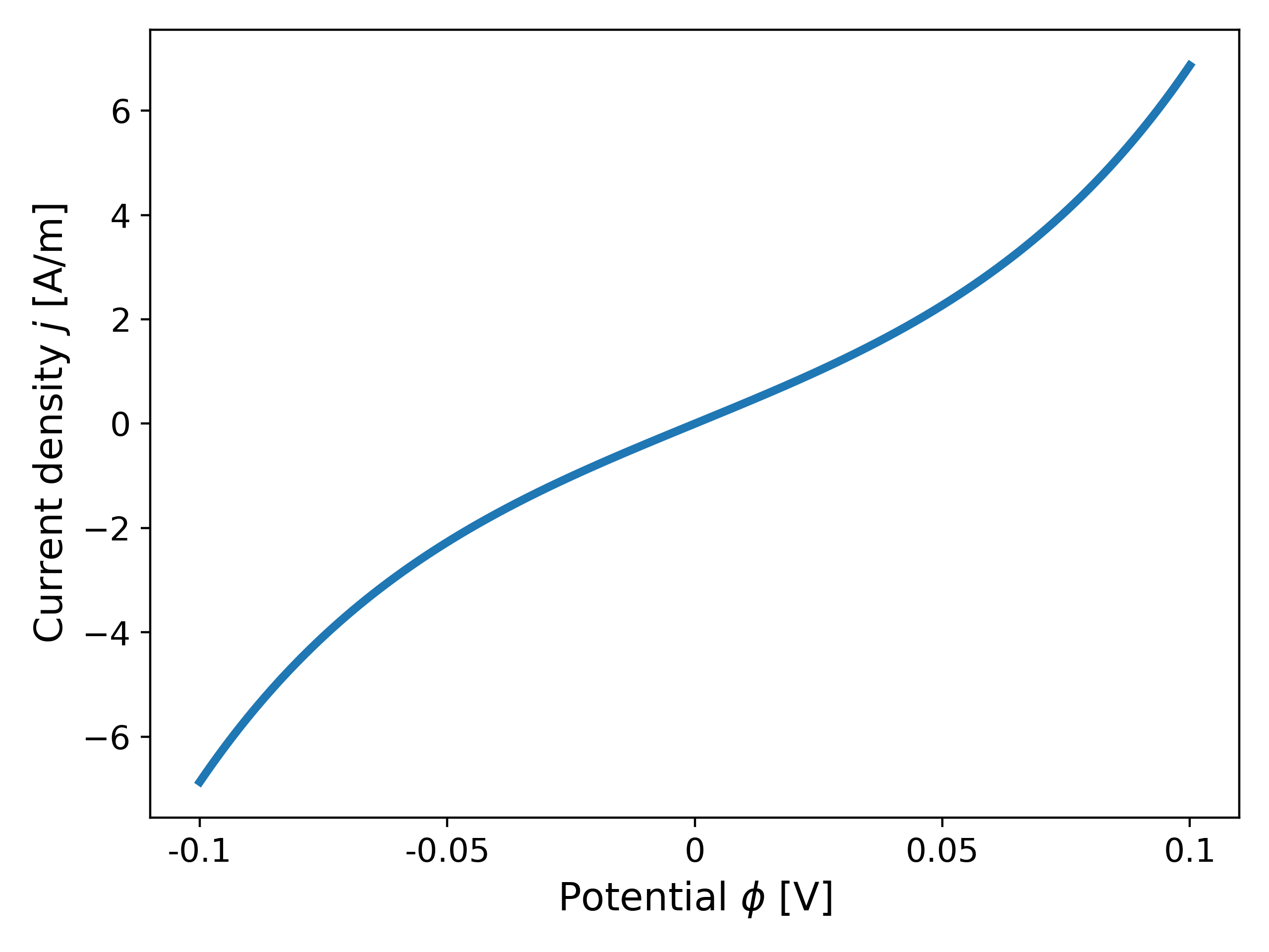
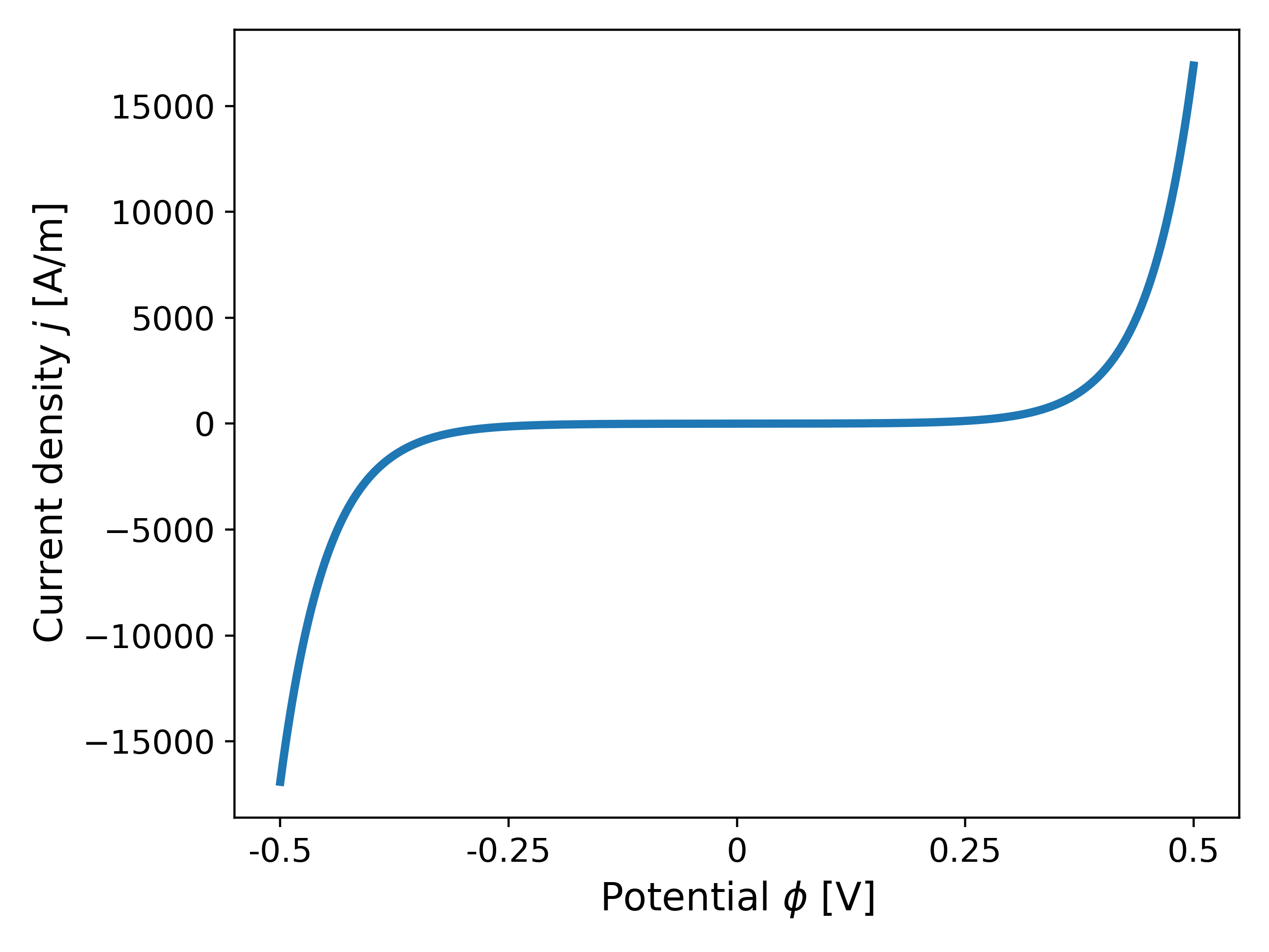
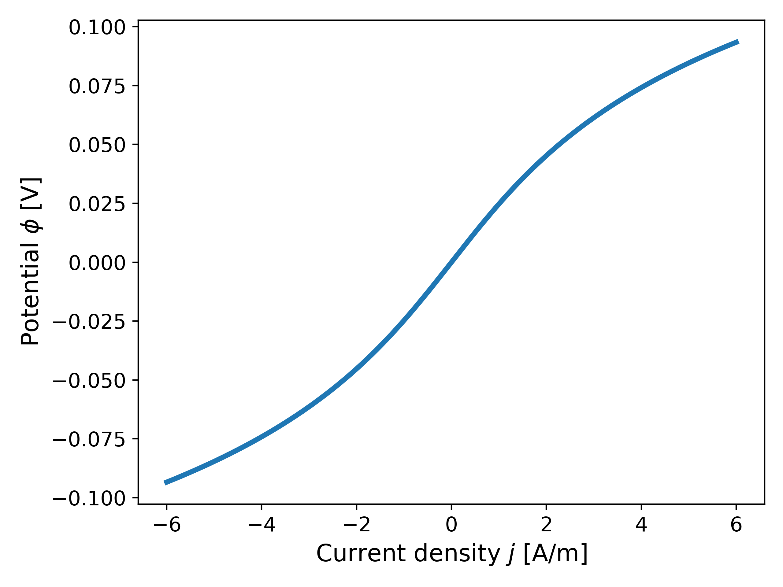
The Butler-Volmer equation is used to model the electrochemical reaction kinetics taking place in electrochemical batteries. In particular, they are used to model the lithium ion exchange between the electrode and electrolyte at the microscopic and macroscopic scale⁴. The equation describes the relationship between the current density $j$ [A/m$^2$] and the electric potential $\phi$ [V] as⁵

\begin{equation} \label{eq:BV} j(\phi) = j_0 \left(e^{\frac{\alpha_a z F}{RT} \phi} - e^{-\frac{\alpha_c z F}{RT} \phi}\right), \end{equation}

where $j_0$ [A/m] is the exchange current density, $\alpha_a$ and $\alpha_c$ [-] are the cathodic and anodic charge transfer coefficients such that $\alpha_a + \alpha_c = 1$, $F \approx 9.648 \times 10^4$ [C/mol] is Faraday’s constant, $R \approx 8.314$ [J/K mol] is the gas constant, $z$ is the number of electrons involved in the electrode reaction (for ex. $z = 1$), and $T$ [K] is the temperature. Fig. 1 shows a plot of the current density as a function of the voltage for commonly chosen physical parameters and $j_0 = 1$ [A/m].

2.1 Example: Solving the Butler-Volmer Equation

We now consider solving the 1D equation

\begin{equation} \label{eq:example_BV} j(\phi) + \sigma \phi = c, \end{equation}

where $\sigma$ [S/m] is the conductivity, and the current density $j$ is described by \ref{eq:BV}. For the purposes of this example, we consider $\sigma = 10^6$ to represent the physical values of most materials⁶. The value of $c$ in the RHS of \ref{eq:example_BV} will be chosen so as to make the solution $\phi_{sol}$ of \ref{eq:example_BV} closer towards $1$ (which increases the gradient of $j$!). The tolerance is set to $\epsilon_{tol} = 10^{-6}$.

We test with multiple values $c \in \{10^5, 5 \times 10^5, 10^6 \}$. We consider an initial guess of $\phi^{(0)} = 0$. The absolute value of the residuals $R = j(\phi) +\sigma \phi - c$ is plotted in Fig. 2 (left) below. The solution for $c = 10^6$ is $\phi_{sol} = 0.6549109190$ and $j_{sol} = 3.450890810218518 \times 10^5$.

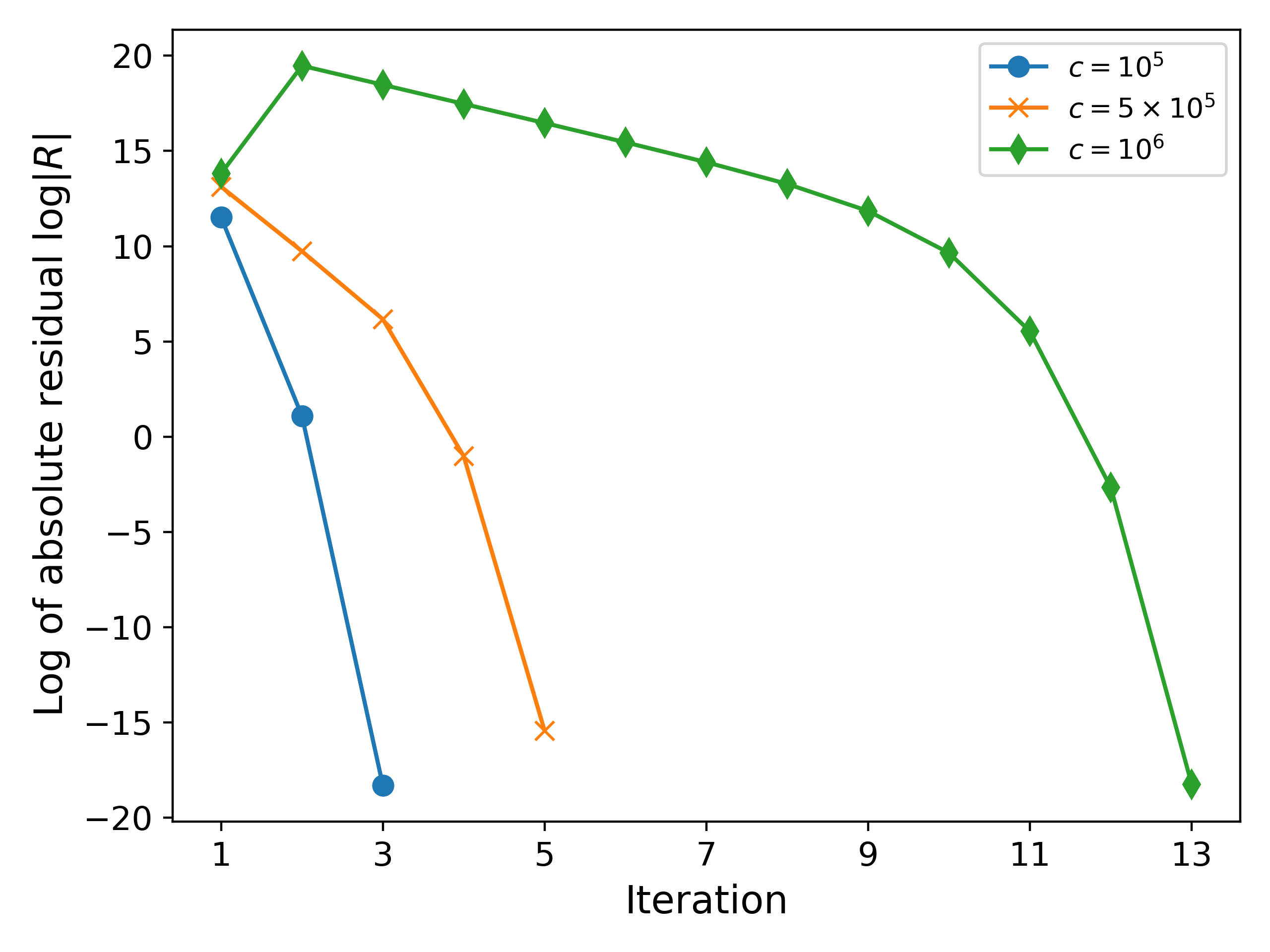
It can be observed that increasing the value of $c$ increases the number of iterations from $3$ to $5$ to $13$. This happens because increasing $c$ increases the potential $\phi$, which further increases the gradient $J$, leading to nondegenerate behaviour.

Note. Equations like \ref{eq:example_BV} are encountered as boundary conditions after spatially discretizing the governing equations using, for example, the finite element or finite volume method. Presently, we do not discuss any numerical discretizations, but will revisit that in a future blog post!

2.2 Example: Slow Convergence for Large Charge Transfer Coefficients

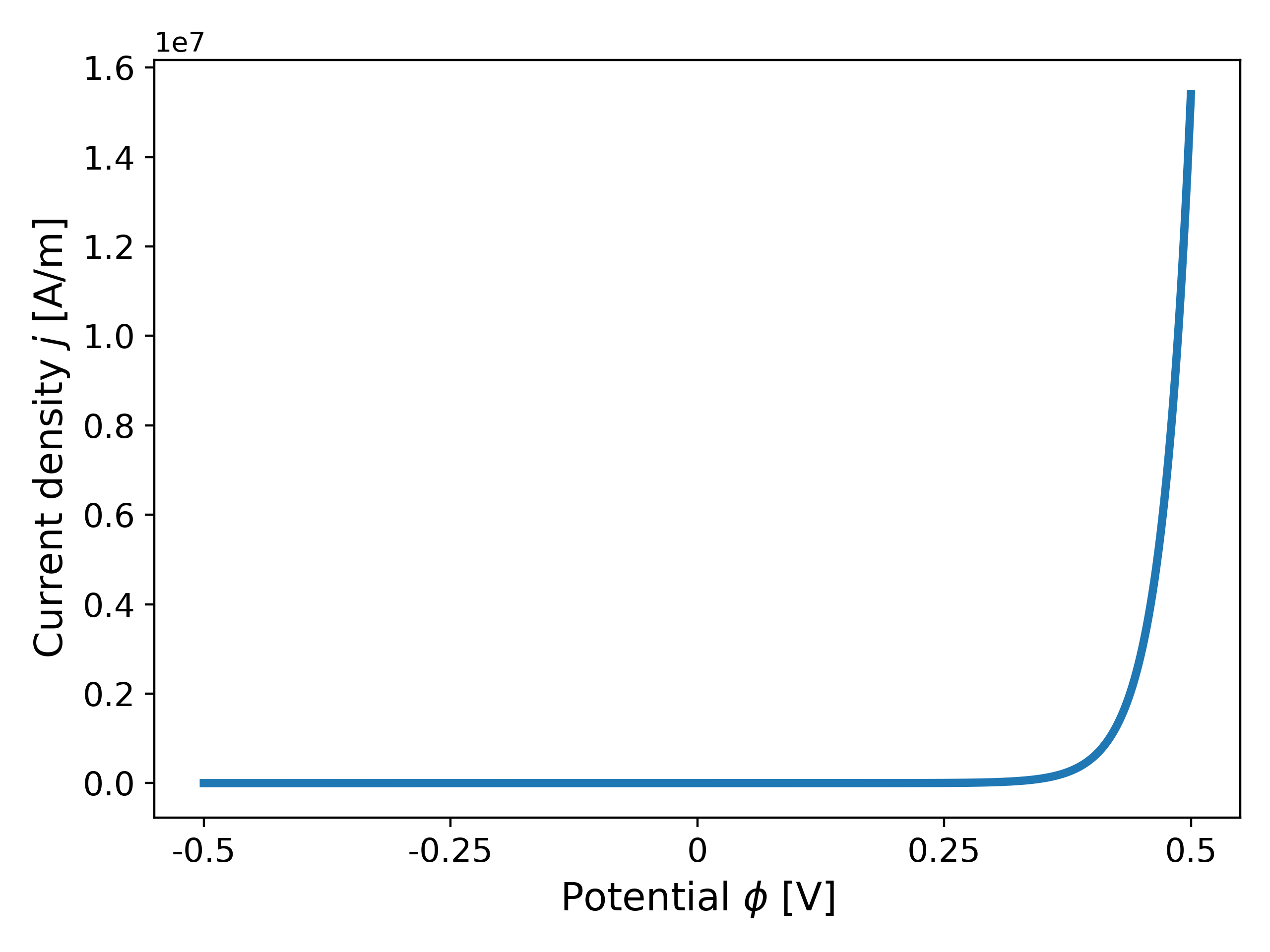
We now consider $\alpha_a = 0.85$ in \ref{eq:BV} in order to test the robustness of Newton’s method; see Fig. 3 below for a plot of the current density. It can be observed that increasing $\alpha_a$ increases the gradients near $\phi = 0.5$.

We now return to solving \ref{eq:example_BV} using $c = 10^6$. In this case, the number of iterations taken by the solver increases to $26$. The reported solution is $\phi_{sol} = 0.4018586997$ and $j_{sol} = 5.981413003436504 \times 10^5$. The convergence can be improved by choosing a different initial guess. For example, for $\phi^{(0)} = 0.5$, the number of iterations taken drops to $9$ and the reported solution is $\phi_{sol} = 0.4018586997$ and $j_{sol} = 5.981413003430553 \times 10^5$; see Fig. 4 for a comparison of the residuals.

2.2 Improving Convergence of Newton’s Method

We now seek to improve the convergence of the Newtons method without having to fine tune our initial guess too much. To this end, we introduce a new formulation of \ref{eq:example_BV} with $j$ as the primary variable as follows: find a solution $j_{sol}$ to

\begin{equation} \label{eq:example_BV_j} j + \sigma \phi(j) = c,
\end{equation}

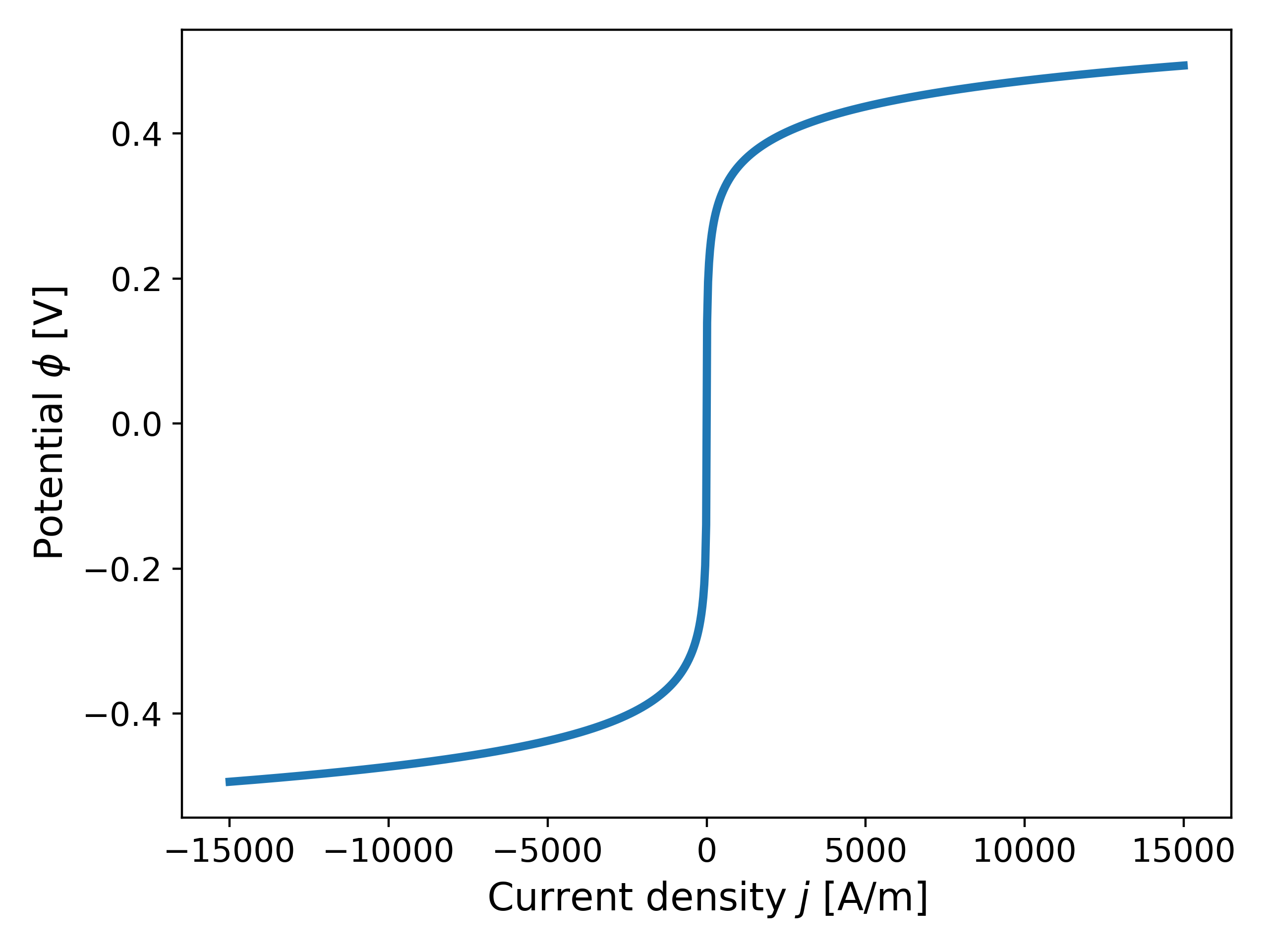
where $\phi(j)$ represents the inverse of $j(\phi)$, i.e., we switch the primary variable from $\phi$ to $j$. Fig. 5 shows a plot of the potential $\phi$ as a function of the current density $j$ using \ref{eq:BV} for $\alpha_a = \alpha_c = 0.5$.

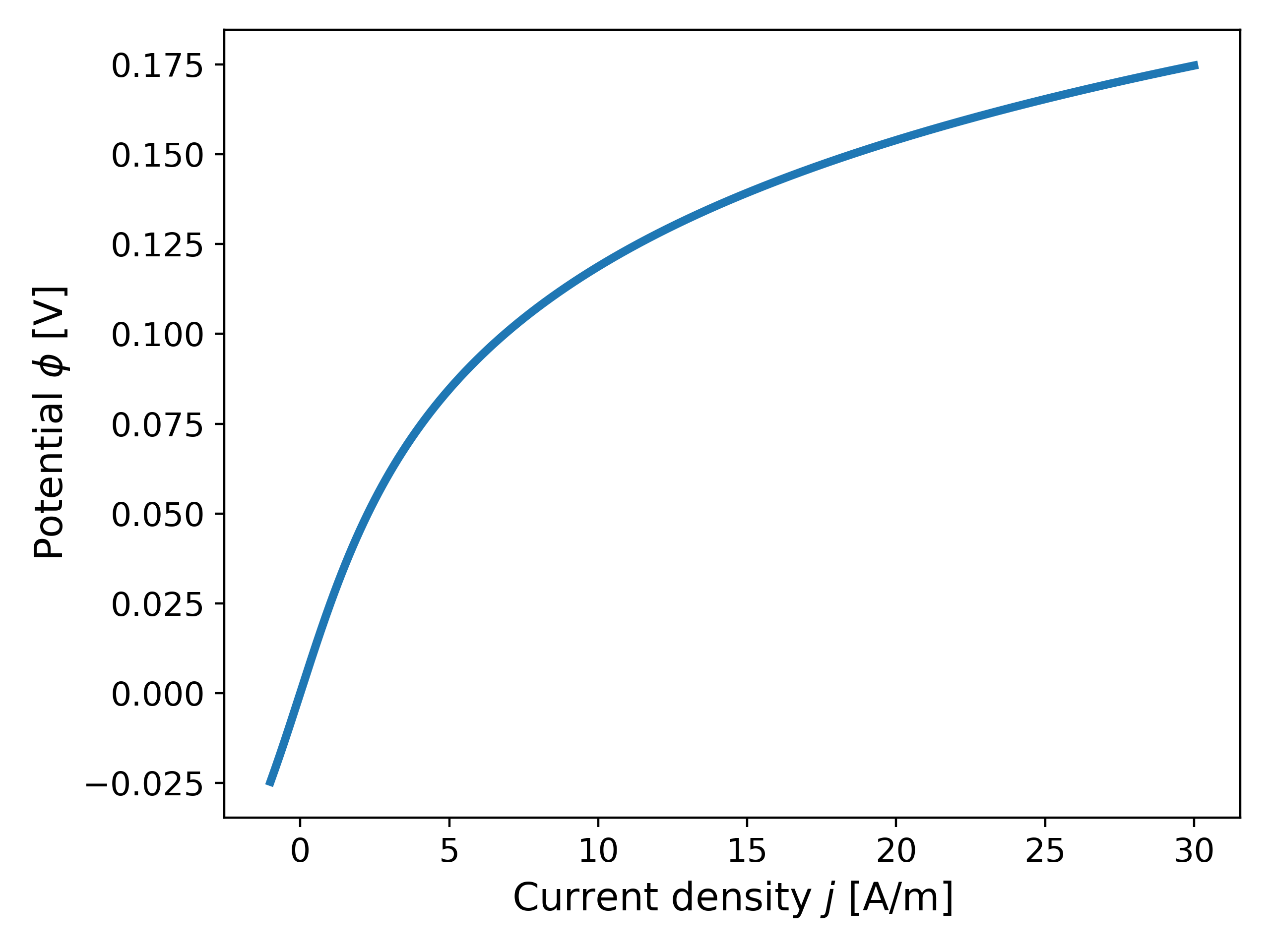
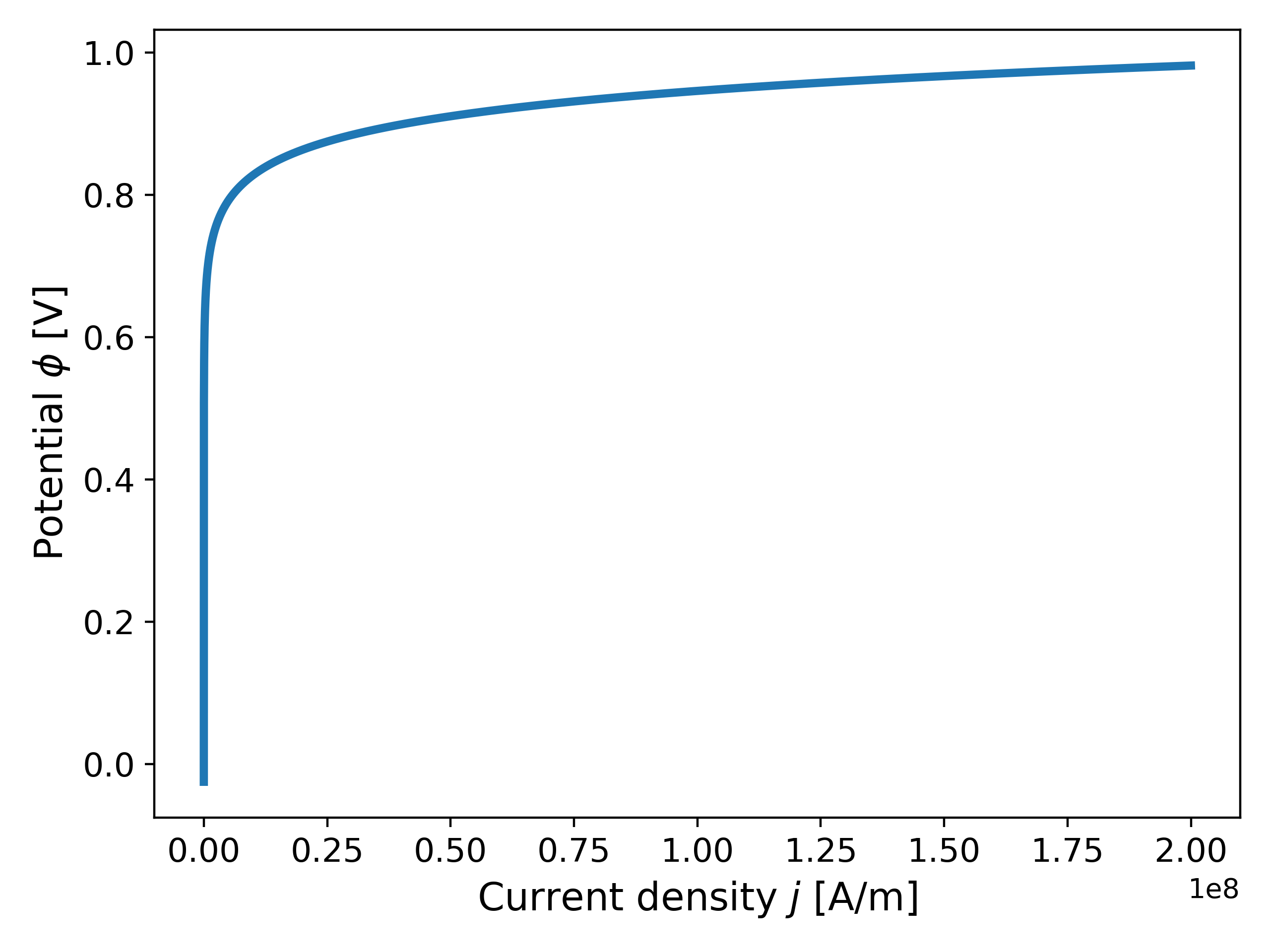
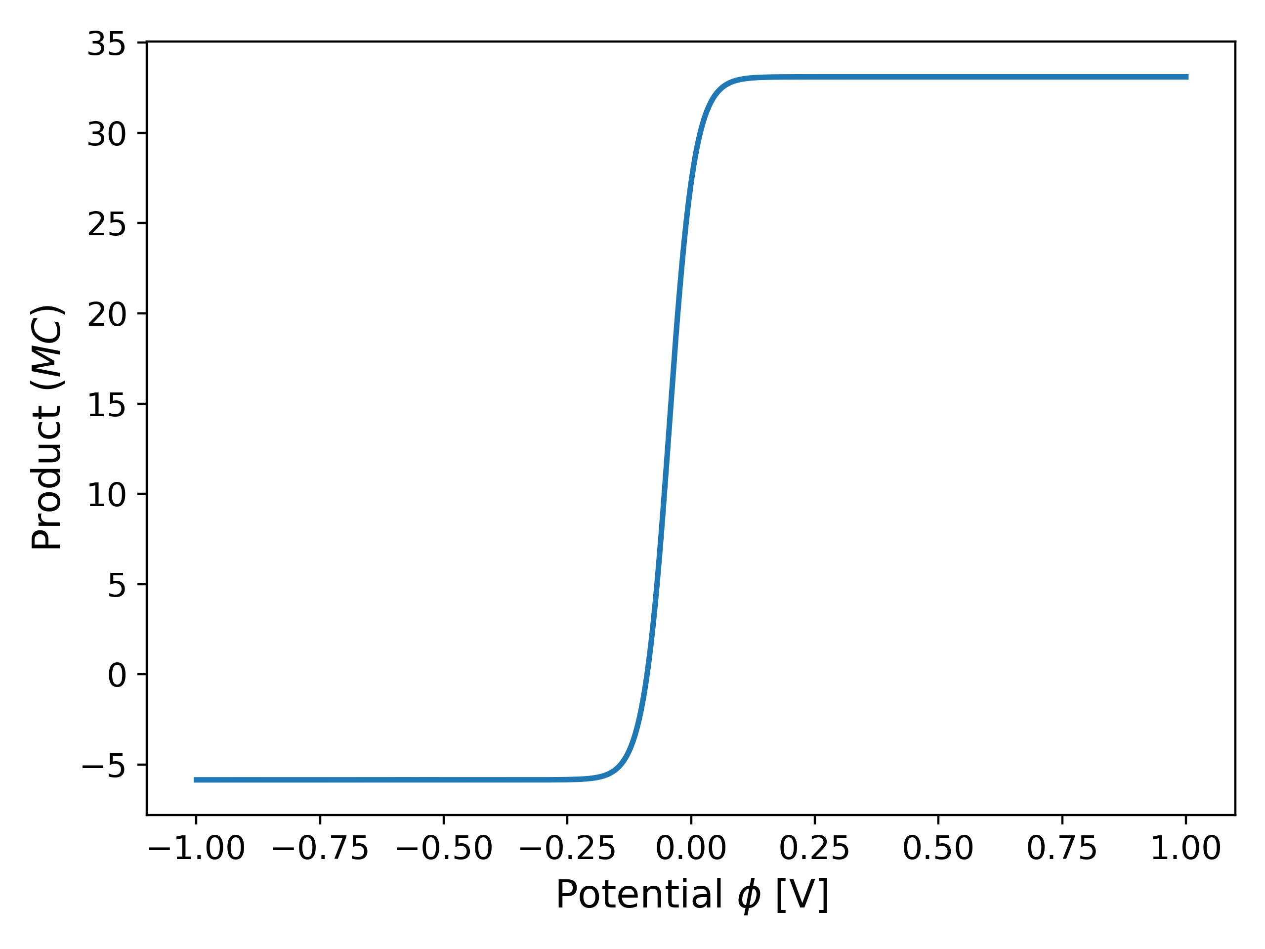
Motivation. We now discuss the motivation for changing our primary variable from $\phi$ to $j$. As observed earlier, when $\alpha_a = 0.85$, the gradient of $j(\phi)$ increases exponentially as $\phi$ increases, but this also implies that the derivative of its inverse, $\phi(j)$, remains bounded and tends to $0$. In particular, for the case of $\alpha_a = 0.85$, the function $\phi(j)$ exhibits concave behaviour with bounded derivatives as $j$ increases, as opposed to $j(\phi)$ as $\phi$ increases as seen in Fig. 3. This is made clear in Fig. 6 below.

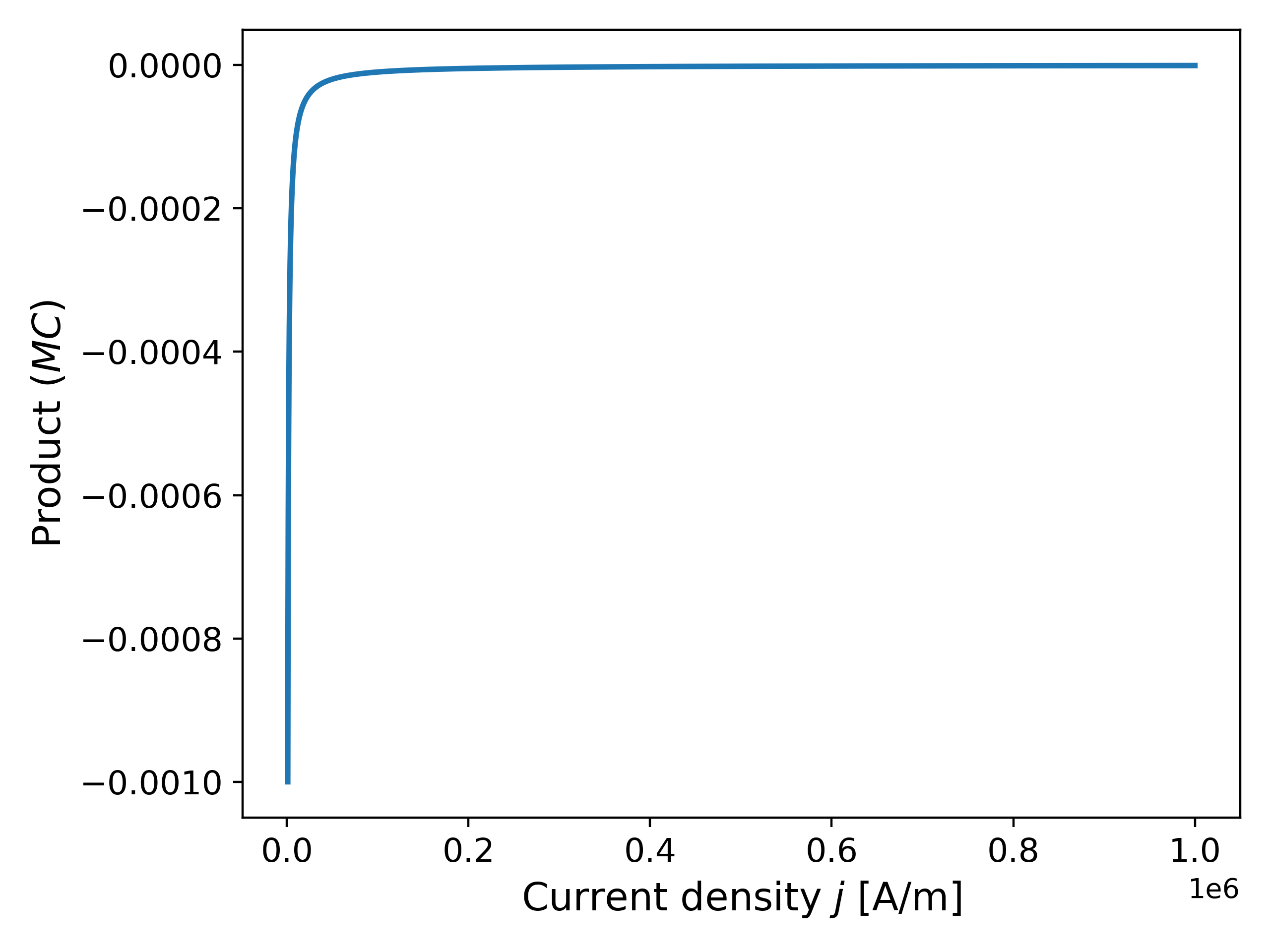
Moreover, computing the product $(MC)$ (as used in \ref{eq:proof4}) for $\phi(j)$ and $j(\phi)$, we observe that the $MC$ is much smaller for $\phi(j)$ near $j = \phi(0.5)$ as opposed to $j(\phi)$ near $\phi = 0.5$; this is shown in Fig. 7 below for convenience (although this may be computed by hand as well!). Thus, from our discussion earlier, we may expect an improvement in the convergence of Newtons method when using $j$ as the primary variable without having to adjust the initial guess too much.

We now solve \ref{eq:example_BV_j} with initial guess $j^{(0)} = \phi(0)$ and $j^{(0)} = \phi(0.5)$ to check if the change in the primary variable improves the convergence of the Newton’s method. The reported solution in both cases are $\phi_{sol} = 0.4018586997$,$j_{sol} = 5.981413003440497 \times 10^5$ and $\phi_{sol} = 0.4018586997$,$j_{sol} = 5.981413003440507 \times 10^5$, respectively. Fig. 8 shows a plot comparing the residuals for different initial guesses comparing the two primary variable approaches.

Indeed, it can be observed that for the case when $j^{(0)} = 0$, the number of iterations have been reduced to from $26$ to $8$. When $j^{(0)} = \phi(0.5)$, the number of iterations taken are also $8$. This example demonstrates the robustness of using $j$ as the primary variable when solving the Butler-Volmer equation.

Note on computing the inverse function $\phi(j)$. The reader may have guessed that the inverse of \ref{eq:BV} does not have a simple analytical expression. Indeed, for our implementation, we have made use of the Ridder method as part of the SciPy library⁷ to aid in computing the inverse $\phi(j)$, i.e., given $j_0 \in \mathbb{R}$, we solve for $\phi_0$ in $j_0 - \phi(\phi_0) = 0$ where $\phi$ is given by \ref{eq:BV}. It may be noted that Newton’s method may be used instead of Ridder method as well without affecting the results presented here.

Further Reading

For an application of the Newton’s method to semismooth function the reader is referred to⁸, where the Newton’s method is used for different formulations of the heat equation. In particular, permafrost (frozen soil for two or more years) have been considered and the robustness of the Newton’s method is shown along with applications of the primary variable switching technique (between enthalpy and temperature), along with proofs of convergence of the method.

References

Michael Ulbrich, Semismooth Newton Methods for Variational Inequalities and Constrained Optimization Problems in Function Spaces, 2011, Mathematical Optimization Society and the Society for Industrial and Applied Mathematics. ↩ ↩2
C.T. Kelley, Iterative Methods for Linear and Nonlinear Equations, 1995, Society for Industrial and Applied Mathematics. ↩
W. Rudin, Principles of Mathematical Analysis, 1976, McGraw-Hill, Inc., 3rd edition. ↩
F. Brosa et al., A continuum of physics-based lithium-ion battery models reviewed, 2022, Progress in Energy, 4. ↩
Gregory L. Plett, Battery Management Systems, Volume 1: Battery Modeling Battery Modeling, 2015, Artech House Publishers. ↩
Electrical Conductivity of some Common Materials, Engineering Toolbox, retreived in 2025. ↩
P. Virtanen et al., SciPy 1.0: Fundamental Algorithms for Scientific Computing in Python, 2020, Nature Methods, 17. ↩
N. Vohra, M. Peszynska, Robust conservative scheme and nonlinear solver for phase transitions in heterogeneous permafrost, 2024, Journal of Computational and Applied Mathematics, 442. ↩