1. Introduction

Non-physical oscillations in numerical solutions are almost always linked to the stability of the underlying numerical method. In time dependent problems, the most well known example is the violation of the Courant–Friedrichs–Lewy (CFL) condition for explicit time stepping methods ¹. The stability for such methods can usually be attained by choosing a small enough time step, which also depends on the spaitial grid size. This however, leads to computationally expensive simulations, requiring more time steps and memory for large time periods. Another way to obtain stability is to use implicit methods, like the backward Euler, which are known to be unconditionally stable. This means that there are no restrictions on the time step size to ensure stability, although a large enough time step comes with loss of accuracy.

Although it is true that implicit methods do not have a time step restriction, choosing a very small time step can lead to a non-monotone system which also produces oscillations. In this blog post, this is what we precisely demonstrate. We consider the well-known heat equation, and show how oscillations can arise for the stable backward Euler time stepping method. We then propose a remedy for these oscillations, and show its robustness in heterogeneous media and higher dimensional settings.

2. Oscillations in Backward Euler for the Heat equation

To motivate the existence of spurious oscillations, we consider the heat equation on $\Omega = (0, 1)$

\begin{equation} \label{eq:heat_eq} \partial_t \left(c \theta \right) - \nabla \cdot \left(k \nabla \theta \right) = f, \; \text{ in } \Omega \times (0, T), \end{equation}

where $\theta$ [$^\circ C$] is the temperature (the primary variable to solve for), $c$ [J/m$^3$ C$^\circ$] is the known volumetric heat capacity of the material, $k = k(x)$ [J/m $^\circ C$ s] is the known thermal conductivity, and $f$ [J/m$^3$ s] is the known external source. Here $T$ [s] denotes the time period. Here we consider homogeneous Dirichlet boundary conditions $\theta(0, t) = \theta(1, t) = 0, \; \forall t \in (0, T)$. Finally, the initial condition $\theta(x, 0) = \theta_0(x)$ is known.

We discretize our system using piecewise-linear Galerkin elements. In particular, let $\Omega_h$ denote the grid for a given spatial grid size $h > 0$ determined by the number of cells in the grid $N_h$ (i.e., $h = {N_h}^{-1}$), let $V_h$ denote the space of piecewise-linear functions, and let $\{\phi_{i + \frac{1}{2}}\}$ denote the basis functions of $V_h$. Following the notation closesly as in our earlier post: Convergence of Solvers and the Importance of Well-posedness, we set up the system in a matrix vector form using implicit time stepping as (with $f = 0$)

\begin{equation} \label{eq:implicit_discretized} M \Theta^n + \tau A \Theta^{n} = M \Theta^{n-1}, \end{equation}

where $\Theta^n \in \mathbb{R}^L$ collects the values of the temperature unknowns at the interior grid points (with $L$ denoting the number of interior grid vertices) at time step $n$, $\tau > 0$ is the time step size, and $M$ and $A$ are the mass and stiffness matrices, respectively. These are defined as

\begin{equation} M_{i, j} = \int_0^1 c \phi_i(x) \phi_j(x) dx, \; A_{i, j} = \int_0^1 k(x) \phi_i(x) \phi_j(x) dx. \end{equation}

It is easy to observe that $M$ and $A$ are symmetric and positive definite (SPD), and have the tri-diagonal $A = \frac{1}{h}$tridiag$(-1, 2, -1)$ and $M = \frac{h}{6}$tridiag$(1,4,1)$ ², where $h>0$ is the grid size.

2.1. A Stability Estimate of the Implicit Euler Scheme

Let the norm $\lVert \cdot \rVert_M$ be defined as $\lVert U \rVert_M = \sqrt{U^T M U}, \; \forall U \in \mathbb{R}^L$. Since $M$ is SPD, it is easy to verify that $\| \cdot \|_M$ is a norm. We prove the following stability estimate.

Lemma 2.1.1. Let $\Theta_0$ be given. Then, for the scheme given by \ref{eq:implicit_discretized}, we have

\begin{equation} \label{eq:theorem_stability} \|\Theta^n \|M \leq \|\Theta{0} \|_M, \; \forall n \geq 1. \end{equation}

The estimate \ref{eq:theorem_stability} essentially guarantees that our numerical solution does not blow up as the time step progressess. Indeed, the $\lVert \cdot \rVert_M$ norm is equivalent to the Euclidean norm using the bounds

\begin{equation} \lambda_{min} \lVert U \rVert_2 \leq \lVert U \rVert_M \leq \lambda_{max} \lVert U \rVert_2, \end{equation}

where $\lambda_{min}$ and $\lambda_{max}$ are the minimum and maximum eigenvalues of $M$, respectively, and $\lVert \cdot \rVert_2$ is the Euclidean norm.

Proof. Taking the inner product of \ref{eq:implicit_discretized} with $\Theta^{n}$, we have

\begin{equation} \label{eq:proof1} (M\Theta^n - M \Theta^{n-1}, \Theta^n) + \tau (A\Theta^n, \Theta^n) = 0. \end{equation}

Noting that since $M$ is symmetric, we have $(M \Theta^n, \Theta^{n-1}) = (M \Theta^{n-1}, \Theta^n)$, and hence we have the identity

\begin{equation} \label{eq:proof2} \left(M(\Theta^n - \Theta^{n-1}), \Theta^n \right) = \frac{1}{2} (M\Theta^n, \Theta^n) - \frac{1}{2} (M \Theta^{n-1}, \Theta^{n-1}) + \frac{1}{2} (M(\Theta^n - \Theta^{n-1}), \Theta^n - \Theta^{n-1}). \end{equation}

Substituting \ref{eq:proof2} into \ref{eq:proof1} gives

\begin{equation} \label{eq:proof3} \frac{1}{2} (M\Theta^n, \Theta^n) + \frac{1}{2} (M(\Theta^n - \Theta^{n-1}), \Theta^n - \Theta^{n-1}) + \tau (A\Theta^n, \Theta^n) = \frac{1}{2} (M \Theta^{n-1}, \Theta^{n-1}). \end{equation}

Now, note that since $M$ and $A$ are SPD, all terms on the LHS of \ref{eq:proof3} are positive, and hence

\begin{equation} \frac{1}{2}(M\Theta^n, \Theta^n) \leq \frac{1}{2} (M\Theta^{n-1}, \Theta^{n-1}). \end{equation}

That is, we have

\begin{equation} \label{eq:proof4} \lVert \Theta^n \rVert_M \leq \lVert \Theta^{n-1} \rVert_M, \; \forall n \geq 1. \end{equation}

By induction, we have our result.

□

Note on the choice of norm. If the matrix $M$ were a diagonal matrix, such as $M = h I$ (as we will obtain later), then the norm $\| \cdot \|_M = h \| \cdot \|_2$. In our experiments, we have also observed the inequality \ref{eq:proof4} to be satisfied by the Euclidean norms. For more stability estimates, the reader is referred to ^{2 3}.

2.2. Homogeneous Media Example

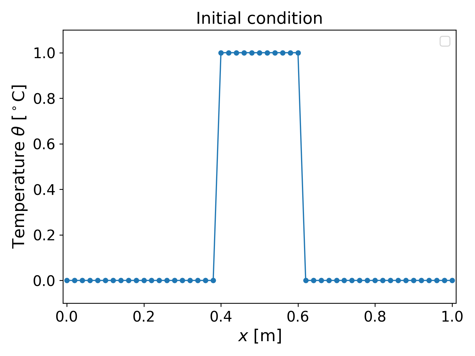
We now consider the cooling of a 1D object $1$ [m] long the middle portion of which is kept at $1$ [$^\circ$C], and the rest at $0$ [$^\circ$ C]. That is, we consider the initial condition

The initial condition is shown in Fig. 1.

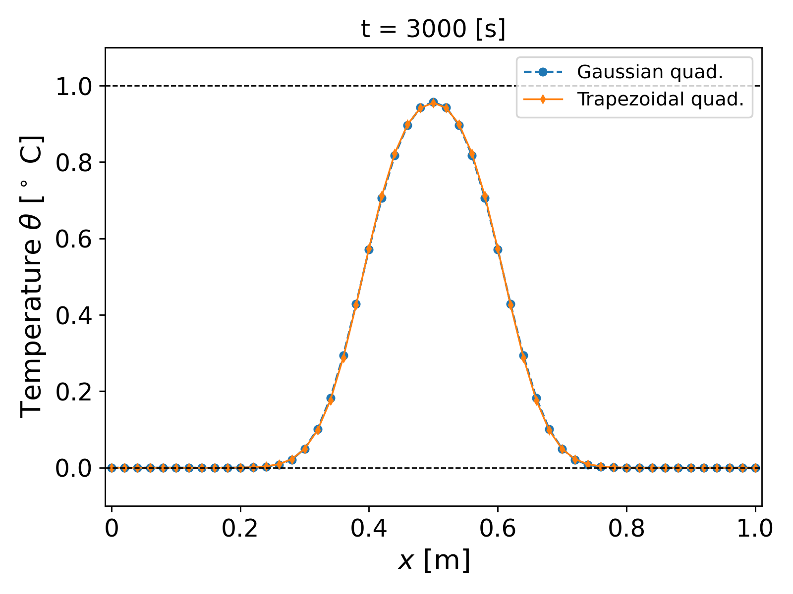
We assume a homogeneous medium and consider material properties similar to water, i.e., we consider $c = 10^6$ [J/ m$^3$ $^\circ$ C] $k = 0.5$ [J/m $^\circ$ C s]. The boundary conditions are as above, i.e., homogeneous Dirichlet. The results for grid size $h = 0.02$ [m] and time step $\tau = 1800$ [s] are shown in Fig. 2.

It can be observed that the temperature profile slowly and smoothly decays as the time progresses, and finally approaches the steady state value of $\theta = 0$.

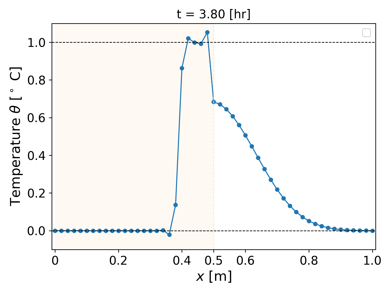
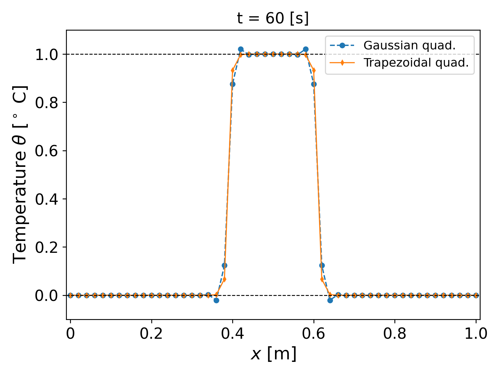
We now test for the robustness of our algorithm. For large time steps, similar temperature profiles as in Fig. 2. are obtained and nothing interesting happens. On the other hand, let us decrease the time step to gauge the temperature profile over smaller time periods. We consider $\tau = 1$ [s], and re-run the simulation over $(0, 2)$ [hr]. The results after a few time steps are shown in Fig. 3.

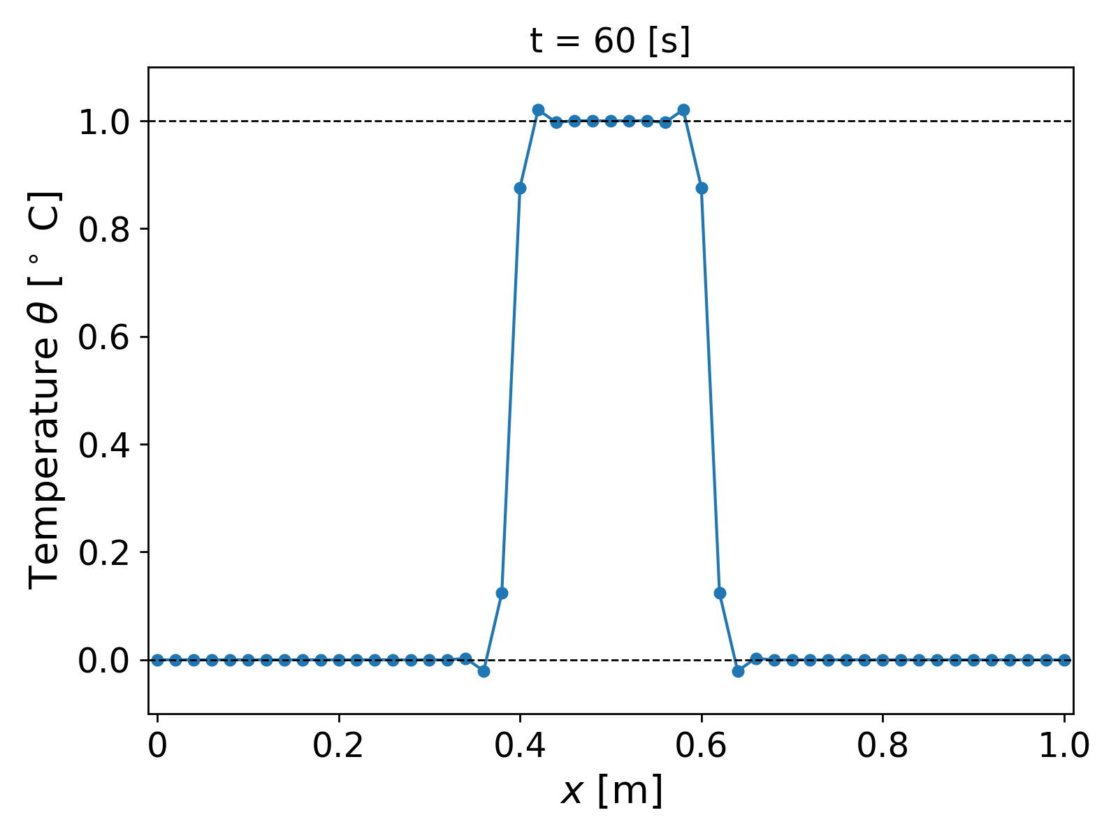
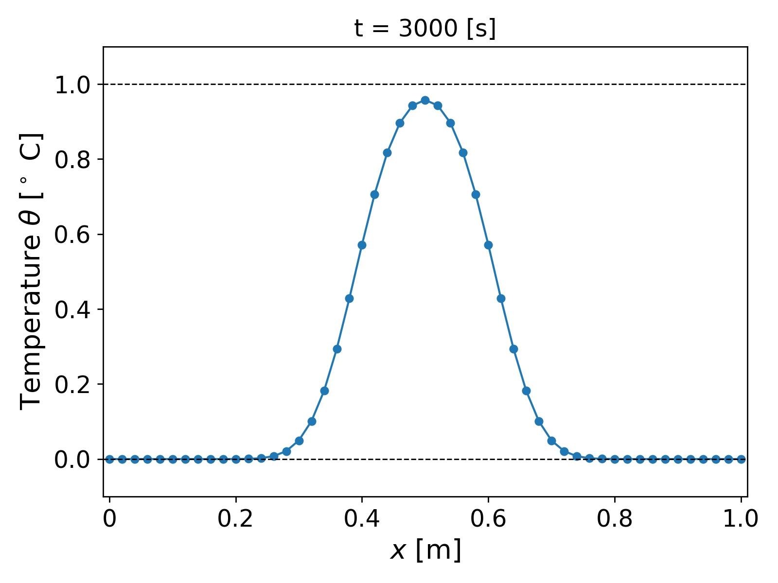
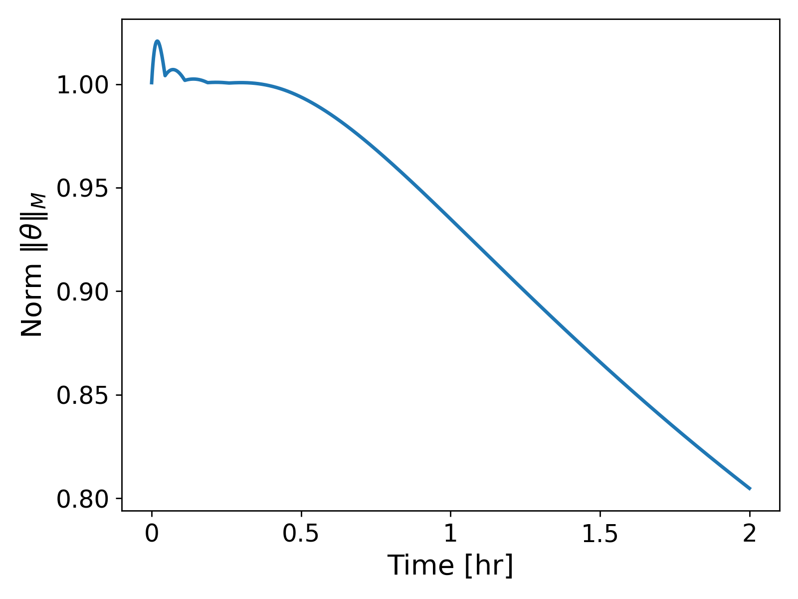
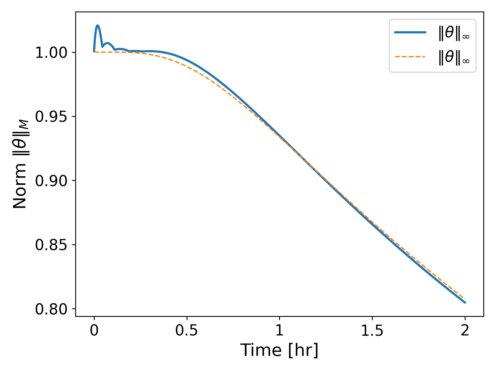
It can be observed that now for the first few time steps, spurious oscillations arise in the temperature profile as shown in Fig. 3. (left). The oscillations lead to the temperature profile over- and undershooting the bounds of the initial temperature profile. That is, the temperature profile at $t = 60$ [s] shows values greater than $1$ [$^\circ$ C] and less than $0$ [$^\circ$ C] being achieved, which lacks physical soundness: indeed, we do not expect the temperature to go higher or lower than the initial state in the absence of any sources or sink terms. The oscillations eventually die out as time progresses, and we get a smooth solution as in the case of $\tau = 3600$. If we look at the $M$-norm values of the temperature, $\| \theta\|_M$, over time, we get a monotonically decreasing curve, as expected from Lemma 2.1.1.; see Fig. 4 (left). We get the same behaviour of the energy norm $\lVert \theta \rVert_2$.

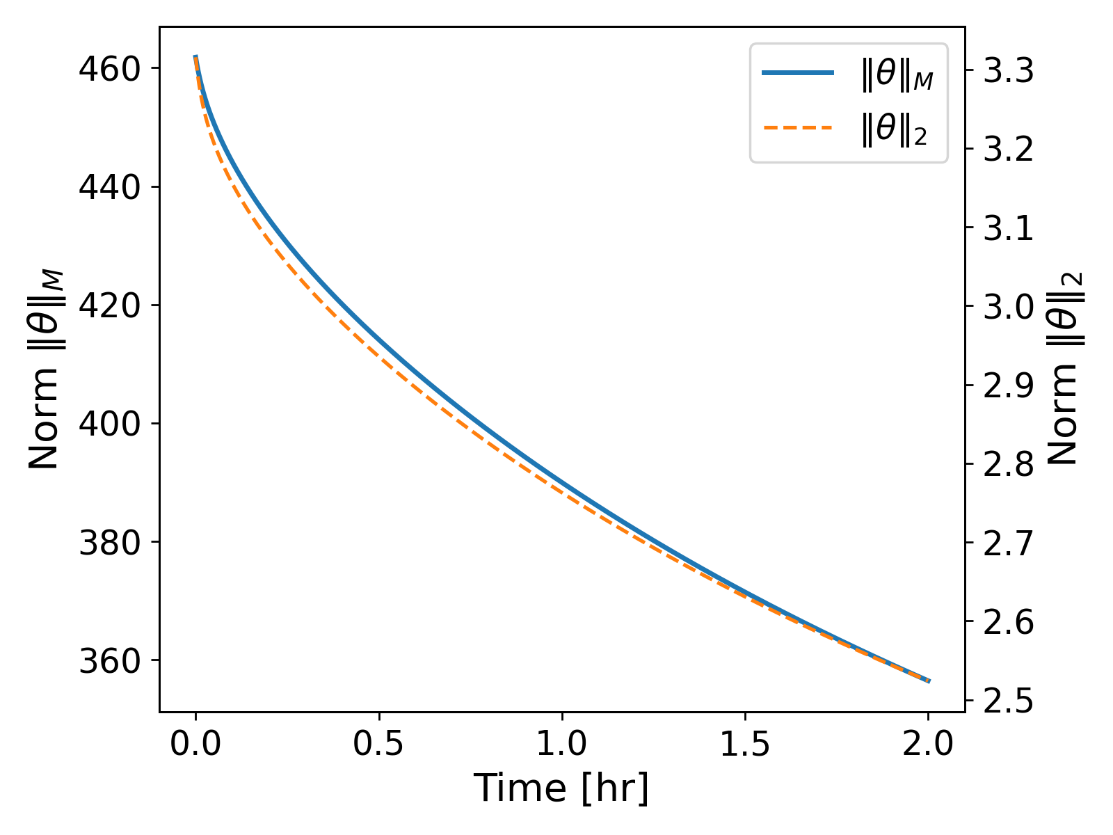
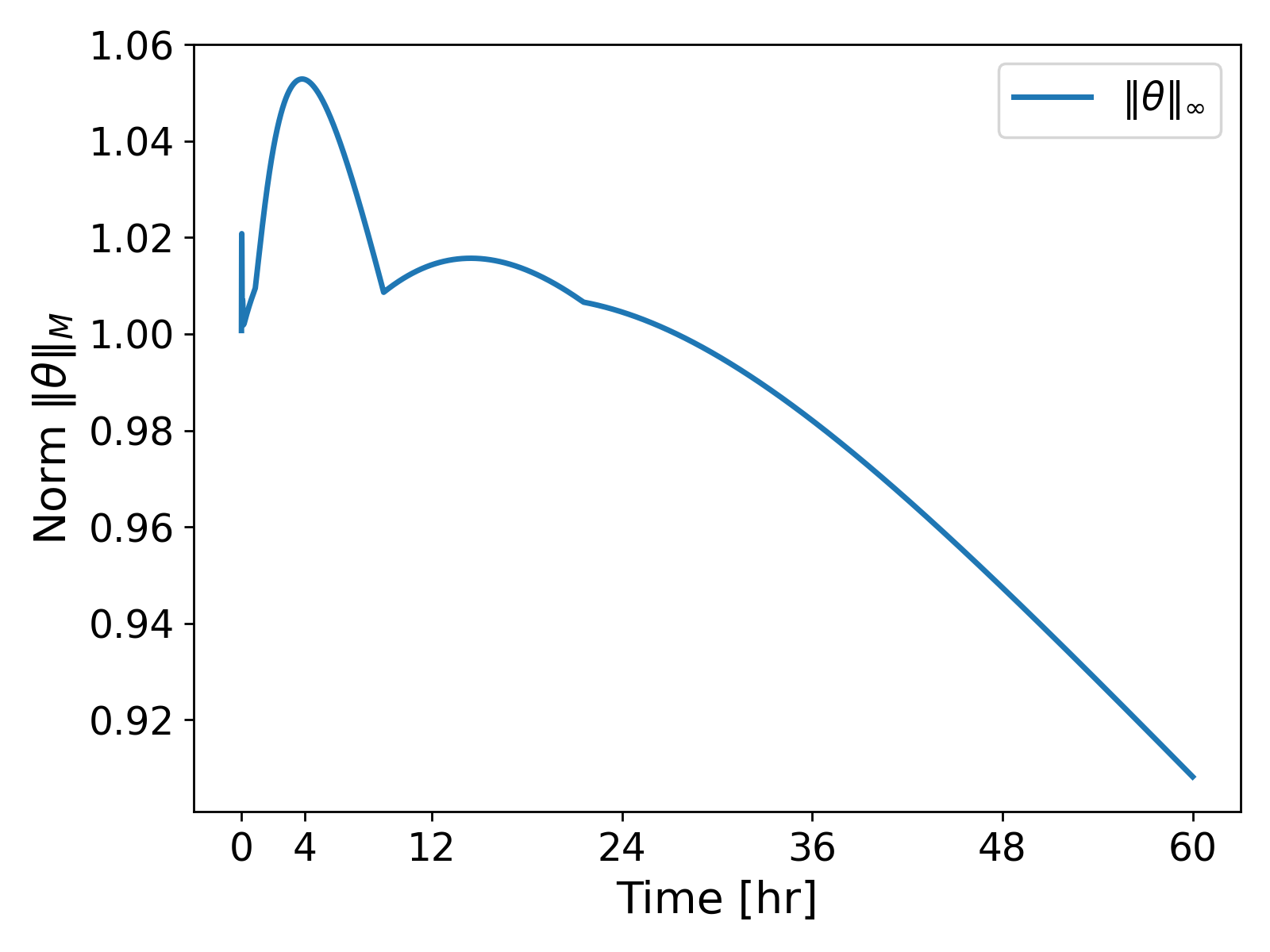
However, the issue becomes easy to spot when we consider the $\lVert \theta \rVert_\infty$ values over the time; see Fig. 4. (right). The plot shows that the values of $\lVert \theta \rVert_\infty$ oscillate towards the beginning of the solution before they start decreasing monotonically. That is, our numerical scheme does not guarantee the boundedness of $\lVert \theta \rVert_\infty$ for all time step sizes $\tau > 0$. The oscillations become more pronounced when we consider heterogeneous media.

2.3. Heterogeneous Media

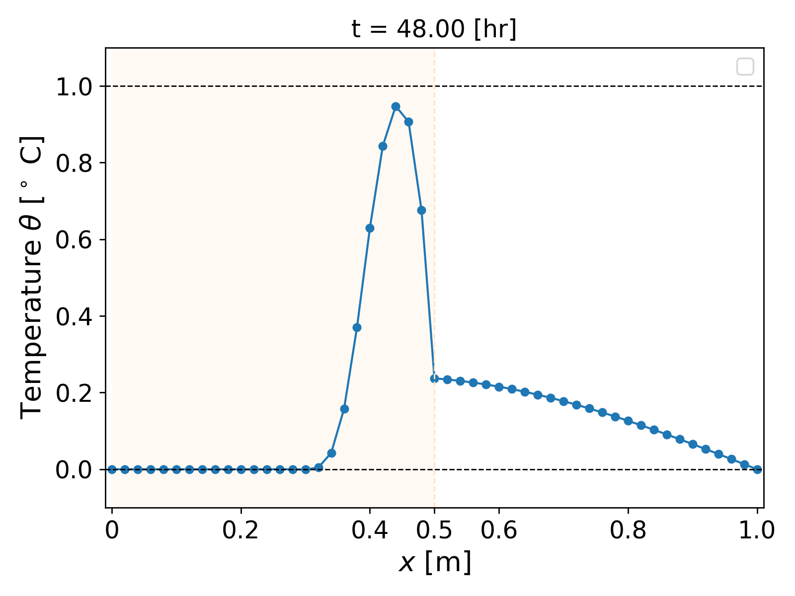
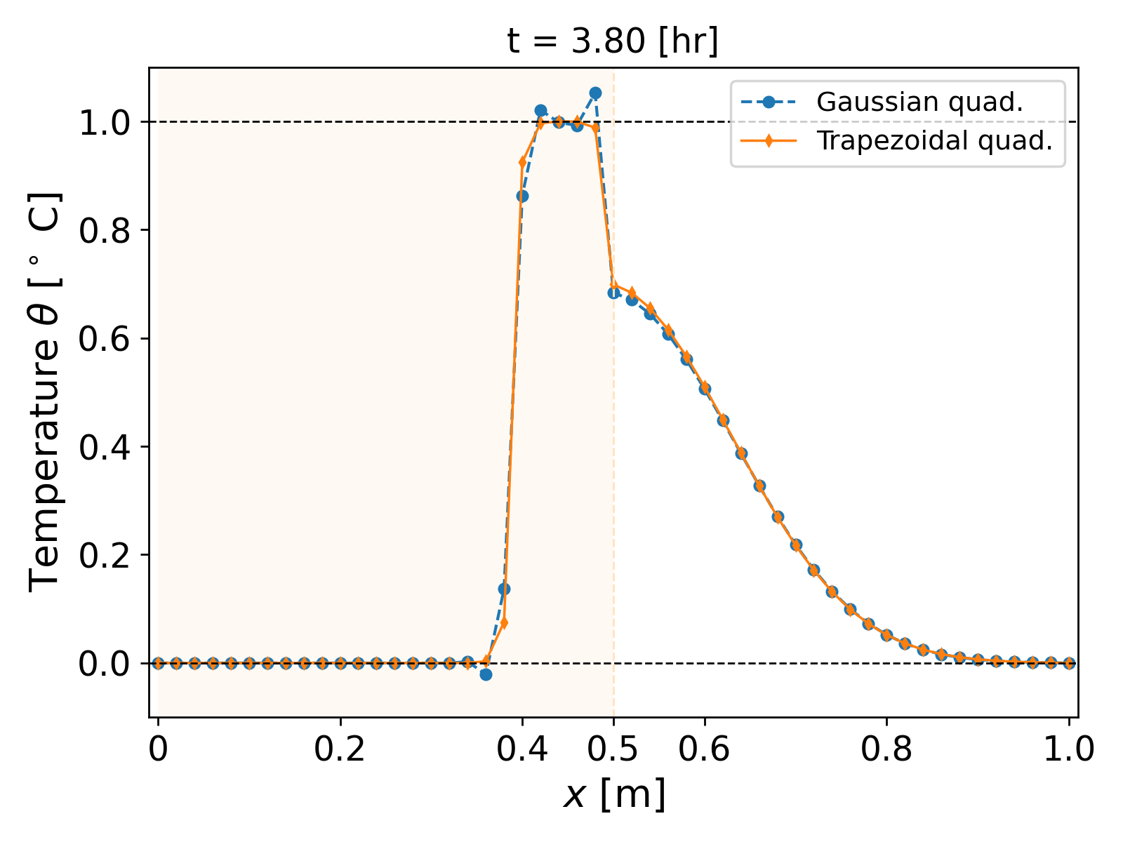
We now re-run our example but using a heterogeneous media. We vary the thermal condutivity as follows

The simulation with a time step of $\tau = 1$ [s] and grid size $h = 0.02$ [m] over a time period of $(0, 60)$ [hr] is shown in Fig. 5. Now in addition to $x = 0.4$ and $x = 0.6$, oscillations also arise near the interface of the heterogeneity, i.e., near $x = 0.5$ [m].

The $\lVert \theta \rVert_\infty$ values over time show the extent of the oscillations polluting the numerical solution; see Fig. 6.

This overshooting and undershooting behaviour of the temperature profile exemplifies a violation of the discrete maximum principle. The issue has been well-studied in literature, and now we analyze the cause of the issue and provide a remedy for the same.

3. M-matrices and Oscillations

A keyword we will be looking at is M-matrices. Let us begin this section with a definition that characterizes M-matrices.

Definition 3.1. A non-singular square matrix $Y \in \mathbb{R}^{L \times L}$ is called an M-matrix if it has non-positive off-diagonal elements and if $Y + D$ is non-singular for each non-negative diagonal matrix $D \in \mathbb{R}^{L \times L}$ ⁴.

A well-known property of M-matrices is positivity of inverses, i.e., for an M-matrix $Y$, we have each entry of $Y^{-1}$ is non-negative. We denote this by $Y^{-1} \geq 0$. This is one of the properties that we are interested in to ensure that our temperature does not undershoot for small time step sizes.

Let us return to our system \ref{eq:implicit_discretized} to see how we can leverage the properties of M-matrices. The matrix $A$ has non-positive off-diagonal and positive diagonal entries (look at its tridiagonal structure). In fact, the matrix $A$ is weakly diagonally dominant (see the next section). The entries of $(M + \tau A)$ are given by (for homogeneous media)

Note that $(M + \tau A + D)$ will always be non-singular for any non-negative diagonal matrix $D$, since $A$ and $M$ are already SPD, and hence $(M + \tau A + D)$ will be SPD. In order for $(M + \tau A)$ to be an M-matrix, we need to ensure that it has non-positive off-diagonal entries. The reader may have already guessed the problem at small $\tau$: as $\tau$ approaches $0$, from \ref{eq:system_entries}, it can be observed that the off-diagonal entries are

\begin{equation} \label{eq:tau_estimate} \left( \frac{ch}{6} - \tau \frac{1}{h}\right) > 0 \end{equation}

and hence $M + \tau A$ ceases to be an M-matrix. Thus, since

\begin{equation} \Theta^n = \left(M + \tau A \right)^{-1} M\Theta^{n-1}, \end{equation}

if $\Theta^{n-1} \geq 0$, then $M\Theta^{n-1} \geq 0$ since $M \geq 0$, however, since $M + \tau A$ is not an M-matrix for small $\tau$, $\left(M + \tau A \right)^{-1}$ may not be positive. From \ref{eq:tau_estimate} the sufficient condition for $\left(M + \tau A\right)$ to be an M-matrix is

\begin{equation} \tau \geq \frac{ch^2}{6k}. \end{equation}

For our homogeneous example above, this gives us a lower bound of approximately $\tau \geq 134$ [s], and thus explains the undershooting of the solution for $\tau = 1$ [s] where the solution $\Theta^n$ dips below zero in Fig. 3.

We now move on to remedy this problem. Let us briefly recap what the issue is: we need a numerical scheme that ensures the solution does not over- or undershoot the bounds set by the initial condition $\Theta_0$. In short, we are looking for a scheme that satisfies an analogue of the maximum principle for parabolic equations.

3.1. Positivity and Bounds Preservation

From the previous section, we have some motivation: we wish to ensure that regardless of our time step $\tau$, the system $\left(M + \tau A \right)$ remains an M-matrix. This will ensure the positivity of the solution. To this end, let us revisit how our mass matrix M is computed. The entries are given by

Since $\{ \phi_i \}$ are piecewise-linear polynomial, we make use of Gaussian quadrature to compute the values \ref{eq:mass_matrix_entry}. Now let us consider an approximation using the trapezoidal rule. This gives

where $\{x_v \}$ are the vertices of the grid $\Omega_h$. That is, the trapezoidal rule gives a diagonal mass matrix $M’ = hI$. This immediately ensures that the system matrix $\left(M’ + \tau A \right)$ has non-positive off-diagonal elements regardless of $\tau$, since $A$ has non-positive off-diagonal elements. Hence, by Definition 1, the matrix $(M’ + \tau A)$ is an M-matrix for any $\tau > 0$. Thus we have $\forall \tau > 0$

\begin{equation} \Theta^{n} = \left(M’ + \tau A \right)^{-1} \Theta^{n-1} \geq 0, \; \text{ if } \Theta^{n-1} \geq 0. \end{equation}

This takes care of the undershooting behaviour by ensuring that the temperature profile does not dip below $0$ [$^\circ$ C]. But what about overshooting? That is, how do we ensure that $\Theta^n$ does not exceed the maximum value of $\Theta^{n-1}$? Thankfully, a stronger bounds preserving result can be obtained for M-matrices. We make use of the following Theorem from ⁵ which gives us an $L^\infty$ bound for our new trapezoidal scheme.

Theorem 3.1.1. Let $Y \in \mathbb{R}^{L \times L}$ be row-wise weakly diagonally dominant, i.e., for $Y = [Y_{i, j}]$

\begin{equation} |Y_{i,j}| \geq \sum_{j \neq i} |Y_{i, j}|, \; \forall i \in {1, 2, \dots, L }. \end{equation}

Then $Y + D$ is an M-matrix for each positive diagonal matrix $D \in \mathbb{R}^{L \times L}$, and $\lVert \left(I + Y \right) \rVert_\infty \leq 1$.

It becomes clear that with the trapezoidal, $\left(M’ + \tau A \right)$ is weakly diagonally dominant, since $A$ is weakly diagonally dominant. This allows us to prove the following Lemma.

Lemma 3.1.2. The solution $\Theta^n$ to \ref{eq:implicit_discretized} when the mass matrix $M’$ is computed using the trapezoidal rule satisfies

\begin{equation} \lVert \Theta^n \rVert \leq \lVert \Theta^{n-1} \rVert, \forall n \geq 1. \end{equation}

Proof The proof follows in a straight forward manner from Theorem 3.1.1. Since $M’ = hI$, we can simply write \ref{eq:implicit_discretized} as

\begin{equation} \left(I + \frac{\tau}{h} A \right) \Theta^n = \Theta^{n-1}, \end{equation}

which gives

\begin{equation} \Theta^n = \left(I + \frac{\tau}{h} A \right)^{-1} \Theta^{n-1}. \end{equation}

By Theorem 3.1.1.,

\begin{equation} \lVert \Theta^n \rVert_\infty \leq \Bigg\lVert\left(I + \frac{\tau}{h} A \right)^{-1} \Bigg\rVert_\infty \lVert \Theta^{n-1} \rVert_\infty \leq \lVert \Theta^{n-1} \rVert_\infty. \end{equation}

This proves the result.

□

Lemma 3.1.2. essentially ensures that our solution does not face the overshooting behaviour as seen before, while the positivity of the solution will ensure no undershooting. Let us demonstrate this by revisiting the examples as earlier. Henceforth we shall call this refer to this scheme which uses $M’$ as the “Trapezoidal quad.” and to the earlier scheme as “Gaussian quad.” scheme.

3.2. Homogeneous Example Revisited

We consider the same parameters as earlier for the homogeneous media example with a time step of $\tau = 1$ [s]. The results are shown in Fig. 7.

It can be observed that the new trapezoidal scheme does not lead to any spurious oscillations, i.e., no over- or undershooting as earlier. In fact, plotting the $|\theta|_\infty$ norm makes clear that the solution in fact remains within the bounds of the initial condition; see Fig. 8.

3.2. Heterogeneous Media Revisited

We now test our new trapezoidal scheme on heterogeneous media. With the same heterogeneous parameters as earlier, we compute the simulation using $\tau = 1$ [s] over a time period of $(0, 60)$ [hr]. The results are shown in Fig. 9.

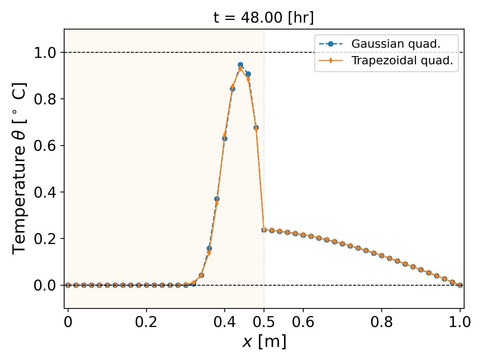
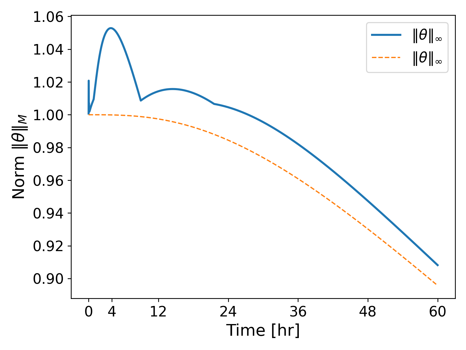
Finally, the $\lVert \theta \rVert_\infty$ plot over time also shows that the values remain bounded as opposed to earlier; see Fig. 10.

3.3. 2D Heterogeneous Media

The above discussion does not restrict itself to 1D. In fact, the same behaviour and remedy works in higher dimensions. Below, we present the results for a 2D simulation of heterogeneous media as illustrated in Fig. 11.

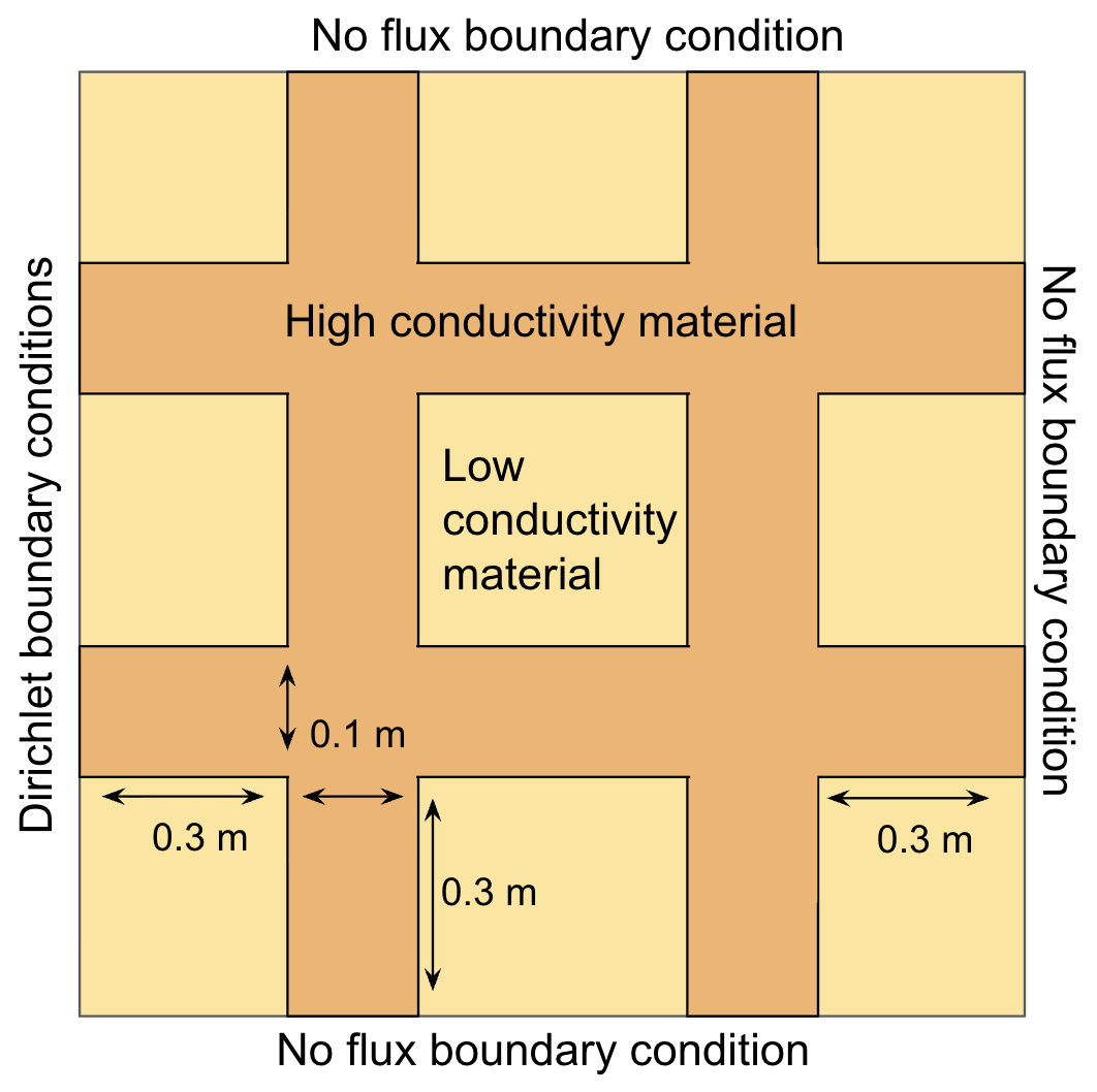
We consdier the domain $\Omega = (0, 1)^2$ [m$^2$]. We choose a low thermal conductivity value of $k = 10^{-4}$ [J/m $^\circ$ C s] and a high thermal conductivity value of $k = 20$ [J/m $^\circ$ C s]. The heat capacity is taken as $c = 10^6$ [J/m$^3$ $^\circ$ C]. The Dirichlet boundary conditions for $\theta(x, y, t)$ are

We run the simulation over $(0, 6)$ [hr] with uniform cells and spatial grid size $10^{-4}$ [m$^2$] and time step size $\tau = 60$ [s]. The results are shown in Fig. 12.

It can be seen that the Gaussian quadrature scheme has a noisy profile, highlighted by the colormap that has been selected such that negative values are represented by blue. Notice that the Gaussian quadature scheme shows negative temperature regions, but the trapezoidal scheme preserves the bounds of the initial condition and the boundary condition. The results demonstrate the robustness of the scheme in 2D. The same has been observed by the author in 3D as well.

Further Reading

The example above highlights the importance of considering all aspects of a numerical scheme, of which stability is inherently indispensable, but so is the behaviour of the solution. This all forms a part of the robustness of the algorithm. Indeed, as is common, one may employ the backward Euler method and adaptive time stepping (which is an extremely common technique for non-linear systems), but if care is not taken in ensuring the scheme is positivity and bounds preservation, spurious oscillations will be sure to pollute the behaviour of the solution. The experienced reader may relate the above to discrete maximum principle and monotnonicity of scheme; see for example ⁶. Another common term for this technique is mass lumping or selective integration, which is widely used in computational mechanics.

The oscillations shown above are not just limited to the heat equation. The author has demonstrated the existence of such oscillations in poroelastic systems as well where mixed finite elements have been used for discretization ⁷. Moreover, for an application of the bounds proved in Lemma 3.1.2. on the convergence of Newton’s method, see ⁸.

References

Randall J. LeVeque, Finite Difference Methods for Ordinary and Partial Differential Equations, SIAM, 2007. ↩
Alexandre Ern, Jean-Luc Guermond, Theory and Practice of Finite Elements, 2004, Springer. ↩ ↩2
Claes Johnson, Numerical solutions of partial differential equations by the finite element method, 1987, Cambridge University Press. ↩
R. J. Plemmons, M-Matrix Characterizations.I - Nonsingular M-Matrices, 1977, Linear Algebra and its Applications (18). ↩
Jurgen Fuhrmann, Existence and uniqueness of solutions of certain systems of algebraic equations with off-diagonal nonlinearity, 2001, Applied Numerical Mathematics. ↩
Daniel Arndt et al., The deal.II library, Version 9.7, Journal of Numerical Mathematics, 2025. ↩
Hao Li, Xiangxiong Zhang, On the monotonicity and discrete maximum principle of the finite difference implementation of C0-Q2 finite element method, 2020, Numerische Mathematik. ↩
Vohra, N. and Peszynska, M., Iteratively coupled mixed finite element solver for thermo-hydro-mechanical modeling of permafrost thaw, 2024, Results in Applied Mathematics (22). ↩
Vohra, N. and Peszynska, M., Robust conservative scheme and nonlinear solver for phase transitions in heterogeneous permafrost, 2024, Journal of Computational and Applied Mathematics. ↩