1. Introduction

In this post, we investigate nonlinear models for mechanics. We start with hyperelasticity equations at their face value, and work on implementing a numerical algorithm to solve the equations. In particular, we look to solve for the displacement $u$ in

where $T$ is the first Piola-Kirchhoff stress tensor for a hyperelastic material, and $f$ is a given force.

We consider St-Venant Kirchhoff materials and make use of the finite element method by first establishing a weak form for the system \eqref{eq:system}. We make clear the challenges that arise as we progress through solving the equations, mostly related to the physical soundness of the solution. As a reference, we also solve the linear elasticity equations to see how the hyperelastic solution profiles look in comparison.

We focus on a simple 1D scenario of deformation due to a constant force (dead load) for a clamped object. We are particularly interested to understand how the displacement profiles for such a simple scenario look for a hyperelastic and linear elastic model. Here we do not necessarily pay attention to the regimes in which the St-Venant Kirchhoff model might be valid or not, but are rather just interested to see how to go about solving the system and understand the challenges that arise from the point of view of numerical solvers.

2. Governing Equations

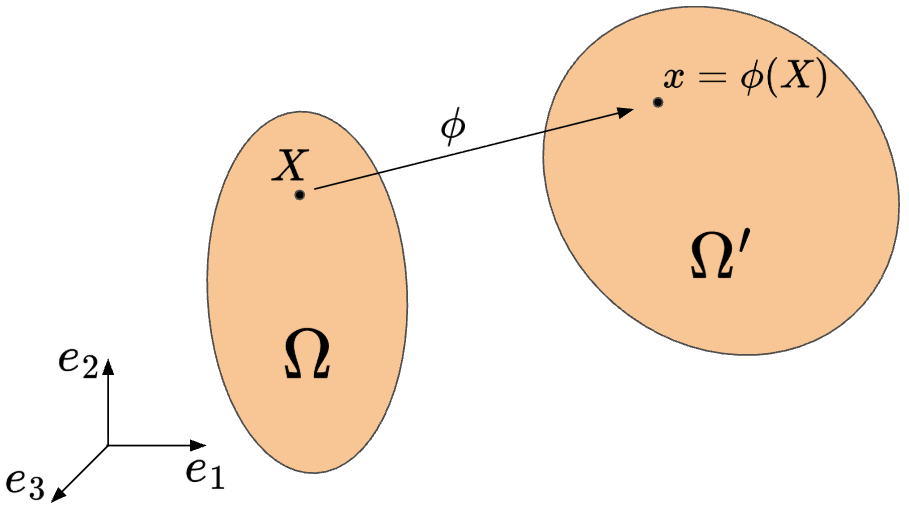
Let the body occupied by $\Omega$ be under some external forces, and let $\Omega’$ denote its deformed configuration (see Fig. 2 for an illustration). Since we wish to solve the system of equations to obtain the displacement field, we consider the system of equations in the reference configuration, and focus on the finite element formulation. The reader is referred to well-known references ^{1 2 3} for an introduction and overview of the system of equations (the list is by no means, even vaguely, exhaustive!). We now provide a brief overview of the system of equations.

2.1. Kinematics

We denote the position of a particle in the reference state $\Omega$ by $X \in \Omega$. In the deformed state, we denote the position by $x = \phi (X) \in \Omega’$, where $\phi : \Omega \rightarrow \mathbb{R}^3$ denotes the deformation, and $\Omega’ = \phi(\Omega)$. The reference and deformed configuration are considered in the same basis denoted by $\{e_1, e_2, e_3 \}$. Further, let $F(X) = \nabla \phi(X) \in \mathbb{R}^{3 \times 3}$ denote the deformation gradient, and let $u(X) = \phi(X) - X$ denote the displacement. Here and below we have $\nabla = \nabla_X$ (with respect to $X$). We also assume that the deformation is orientation preserving, i.e., det$\nabla \phi > 0$ in $\Omega$.

We denote the right Cauchy-Green strain tensor by $C = F^T F$, and the Green-St-Venant strain tensor by $E = \frac{1}{2}\left( C - I \right)$, where $I \in \mathbb{R}^{3 \times 3}$ is the identity matrix. This gives us

Finally, the linearized strain is given by $\epsilon = \frac{1}{2}\left(\nabla u + \nabla u^T \right)$, and it can be seen that $\epsilon \approx E$ for small displacements $u$.

2.2. Equilibrium Equations

For a pure displacement problem, under an external body force $f : \Omega \rightarrow \mathbb{R}^3$, the equation of equilibrium in the reference configuration is given by [Ciarlet’ 1988, Theorem 2.6-1] ¹

where $T : \Omega \rightarrow \mathbb{R}^3$ is the second order stress tensor, and in particular the first Piola-Kirchhoff stress tensor. We complete the system \eqref{eq:stress_eq} with homogeneous Dirichlet boundary conditions

We now list the constitutive relations for the first Piola-Kirchhoff stress tensor.

2.2.1. Hyperelasticity: St-Venant Kirchhoff Material

In this post, we consider the simplest constitutive relation for a hyperelastic material, the St-Venant Kirchhoff relation. For the St-Venant Kirchhoff material, the first Piola-Kirchhoff stress tensor is given by ¹

where $\lambda \in \mathbb{R}$ and $\mu \in \mathbb{R}$ are Lamé parameters related to the Youngs modulus $E_Y \in \mathbb{R}$ and Poisson ratio $\nu \in \mathbb{R}$ by

Note on the choice of the St-Venant Kirchhoff material. It can be shown that the St-Venant Kirchhoff material is not the most sound way of approximating physically observed material behavior. Indeed, it can be shown that such a material, i.e., where the the stress relation is given by \eqref{eq:st_venant_fpks}, can undergo extreme deformation to arbitrarily small volumes by expending finite energy. This is physically inconsistent with natural materials, and better choices instead of \eqref{eq:st_venant_fpks} include Neo-Hookean materials, Ogden etc. ^{1 3} Here we make use of \eqref{eq:st_venant_fpks} due to its simple form.

2.2.2. Linear Elasticity

In the linear elastic framework, the first Piola-Kirchhoff stress tensor is given by ¹

2.3. Weak Formulation and Existence of Solution

We now present the weak formulation for \eqref{eq:stress_eq}-\eqref{eq:Dirichlet_boundary}. Here, we seek the solution $u \in H_0^1(\Omega)$. The continuous weak formulation is as follows: find $u \in H_0^1(\Omega)$ such that ¹, [Oden’ 1979, Eq. 7.1] ⁴,

where $:$ is the contraction operator between two tensors defined as $A : B = \sum_{i, j = 1}^{M} A_{i,j} B_{i, j}$ for any two $A, B \in \mathbb{R}^{M \times M}$. The existence of a solution to \eqref{eq:continuous_weak_form} is established using the implicit function theorem in [Ciarlet’ 1988, Theorem 6.4-1] for the St-Venant Kirchhoff material \eqref{eq:st_venant_fpks}, and using Gårding operators in [Oden’ 1979, Theorem 7.1] under more regularity assumptions.

We now present the fully discrete formulation. In this post, we focus on 1D, and on $P_1$ elements. Let $\Omega = (0, 1)$, and let $\Omega$ be divided into $M$ cells $(X_{j}, X_{j+1})$, $0 \leq j \leq M-1$, of uniform width denoted by $h = \frac{1}{M}$. Let $V_h$ is the subspace of piecewise-linear functions with basis functions given by

The fully discrete form of \eqref{eq:continuous_weak_form} reads as follows: find $u_h \in V_h$ such that

Existence of solution. Before we set up a numerical experiment, we first prove the existence of a solution to \eqref{eq:discrete_weak_form} for appropriate forces $f$. We rewrite \eqref{eq:discrete_weak_form} as

where $U \in \mathbb{R}^{M-1}$ collects the entries of $u_h = \sum_{j} U_j \phi_j$, i.e., $U = [U_1 \; U_2 \; \dots \; U_{M-1}]^T$, and $\mathcal{T} : \mathbb{R}^{M-1} \rightarrow \mathbb{R}^{M-1}$ is a nonlinear map with entries

and the vector $L_f \in \mathbb{R}^{M-1}$ collects the entries

We now present a little existence result.

Theorem 2.3.1. Let $f \in C^0(\Omega)$. Then, for $\lVert f \rVert_\infty$ small enough, there exists a solution to \eqref{eq:nonlinear_map_eq}.

Proof. We make use of the inverse function theorem. First note that

is a polynomial in $\left(U_1, U_2, \dots, U_{M-1} \right)$, $\forall 1 \leq i \leq M-1$. For example, by definition, since $E(u_h) = \frac{1}{2}(F(u_h)^2 - 1)$, we have for $1 < i < M-1$

and since

it can be easily seen that $\mathcal{T}_i$ is a polynomial and its continuity and smoothness follows.

Now, note that, for $U = 0$ (here we mean $0 \in \mathbb{R}^{M-1}$), we have $\mathcal{T}(U) = 0$. We now compute the Jacobian $\mathcal{J}$ of $\mathcal{T}$

Since $u_h = \sum_j U_j \psi_j$, by the chain rule, we have

For $U = 0$, we have $F(u_h) = 1$, and thus we have from \eqref{eq:proof_jacobian} that $\mathcal{J}(0) = \frac{\left(\lambda + 2\mu \right)}{h}\text{tri}(-1, 2, -1)$ is a tri-diagonal matrix and is symmetric positive definite. Hence $\mathcal{J}(0)$ is invertible. Thus, by the inverse function theorem ⁵, $\exists$ open neighborhoods $R_1, R_2 \subset \mathbb{R}^{M-1}$ $0 \in R_1$, $0 \in R_2$, $\mathcal{T}$ is one-one on $O_1$, and

That is, for any $f \in R_2$, i.e., if $\lVert f \rVert_\infty$ is small enough, $\exists U_f \in R_1$ such that $\mathcal{T}(U_f) = f$. This completes the proof.

□

The above result does not prove the existence of solutions for any arbitrary $f$ but in our numerical experiments we have obtained solutions for large $\lVert f \rVert_\infty$.

A crucial point to consider now is how we still have not mentioned uniqueness for our hyperelastic system. For linear elasticity, both uniqueness and existence is well-established and follows from Korn’s inequality ^{1 6}, but for hyperelastic system this is not the case. As we shall explore below, uniqueness for hyperelastic systems indeed isn’t guaranteed and leads to non-physical results.

3. Numerical Experiments

We now discuss the numerical implementation and simulate the physical scenario described in the Introduction.

3.1. Nonlinear Solver and Implementation Details

We now describe the details of our numerical implementation. We make use of Newton’s method to solve the system \eqref{eq:nonlinear_map_eq}. Starting with an initial guess $U^{(0)}$, we iterate as follows ⁷:

We perform the Newton step till we obtain convergence of the residuals $\lVert \mathcal{T}(U^{(m-1)}) - L_f \rVert_\infty < \epsilon_{rel, tol}$ or $\lVert \delta U^{(m)} \rVert_\infty < \epsilon_{tol}$, for some prescribed tolerance $\epsilon_{abs, tol} > 0$. In our simulations, we use $\epsilon_{abs, tol} = 10^{-12}$ and $\epsilon_{rel, tol} = 10^{-14}$.

Since we are using $P_1$ elements for the displacement $u$, this means that $F$ is a piecewise-constant on each grid cell. This makes numerical integration straightforward when computing the Jacobians of $\mathcal{T}$. Indeed, from \eqref{eq:proof_jacobian} we have for an interior $1 < i < <M-1$

The implementation is done using the Python library Numpy ⁸.

3.2. Numerical Experiment: Deformation Under Dead Load

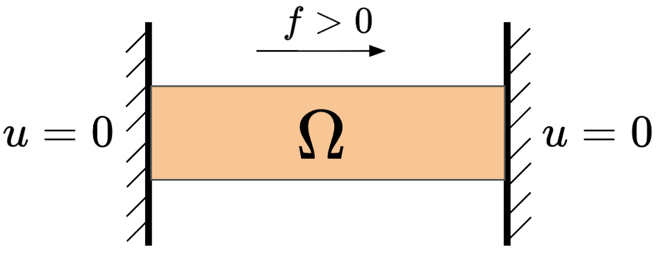
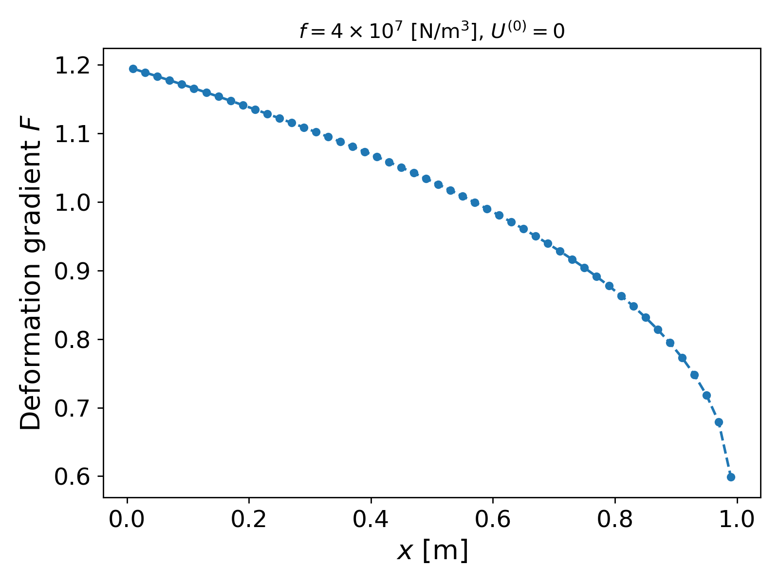
We now consider a physical scenario as shown in Fig. 1 with a homogenous material occupying $\Omega = (0, 1)$ [m] with $E_Y = 10^7$ [Pa] and $\nu = 0.48$ [-] to mimic the properties of rubber ⁹. We consider $f \in \{10^6, \; 4 \times 10^7 \}$ [N/m$^3$] to demonstrate the performance of the solver for small and large displacements. We simulate using a grid size of $h = 0.05$ [m]. We use an initial guess $U^{(0)} = 0$. The results are shown in Fig. 3.

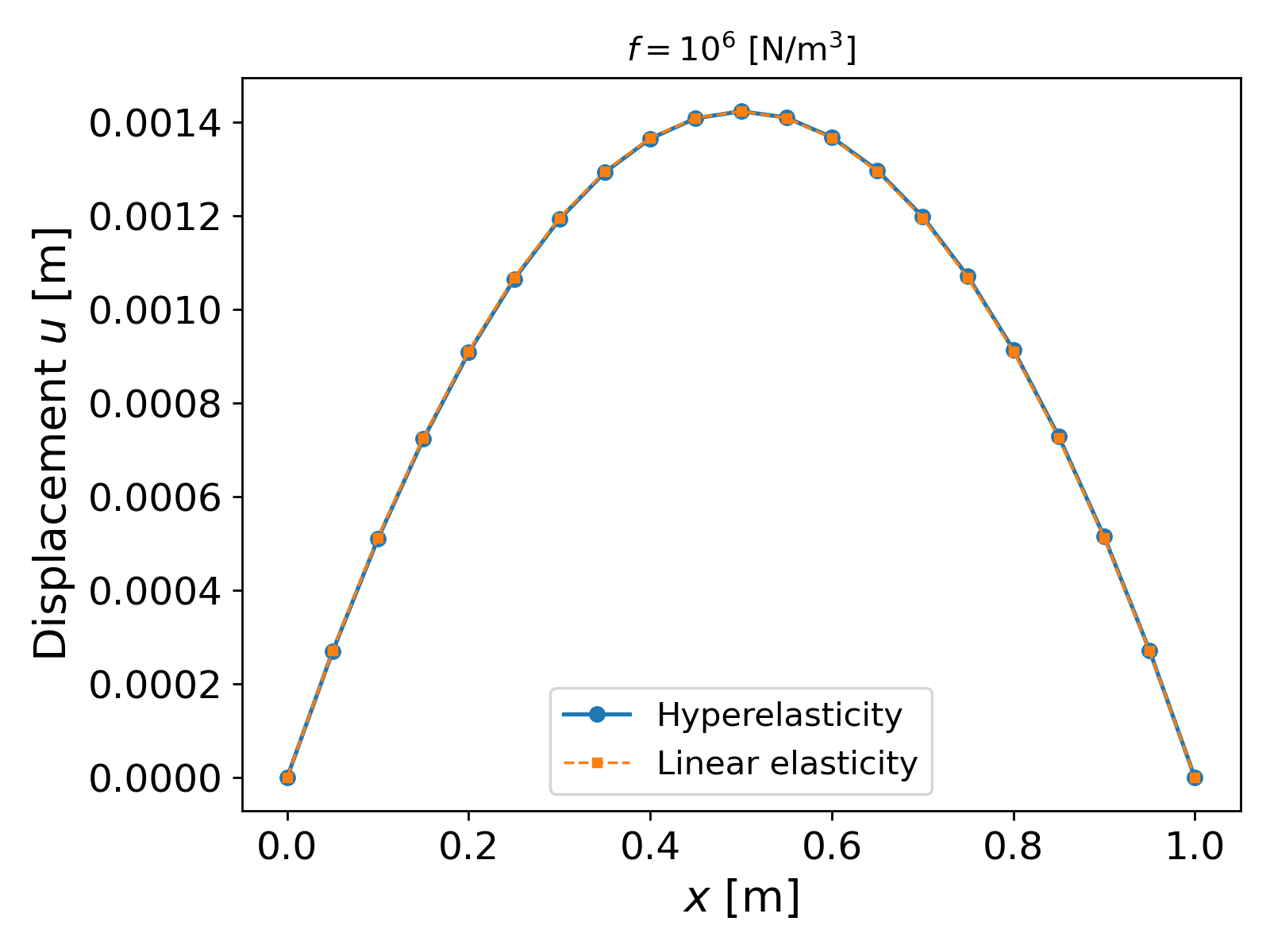
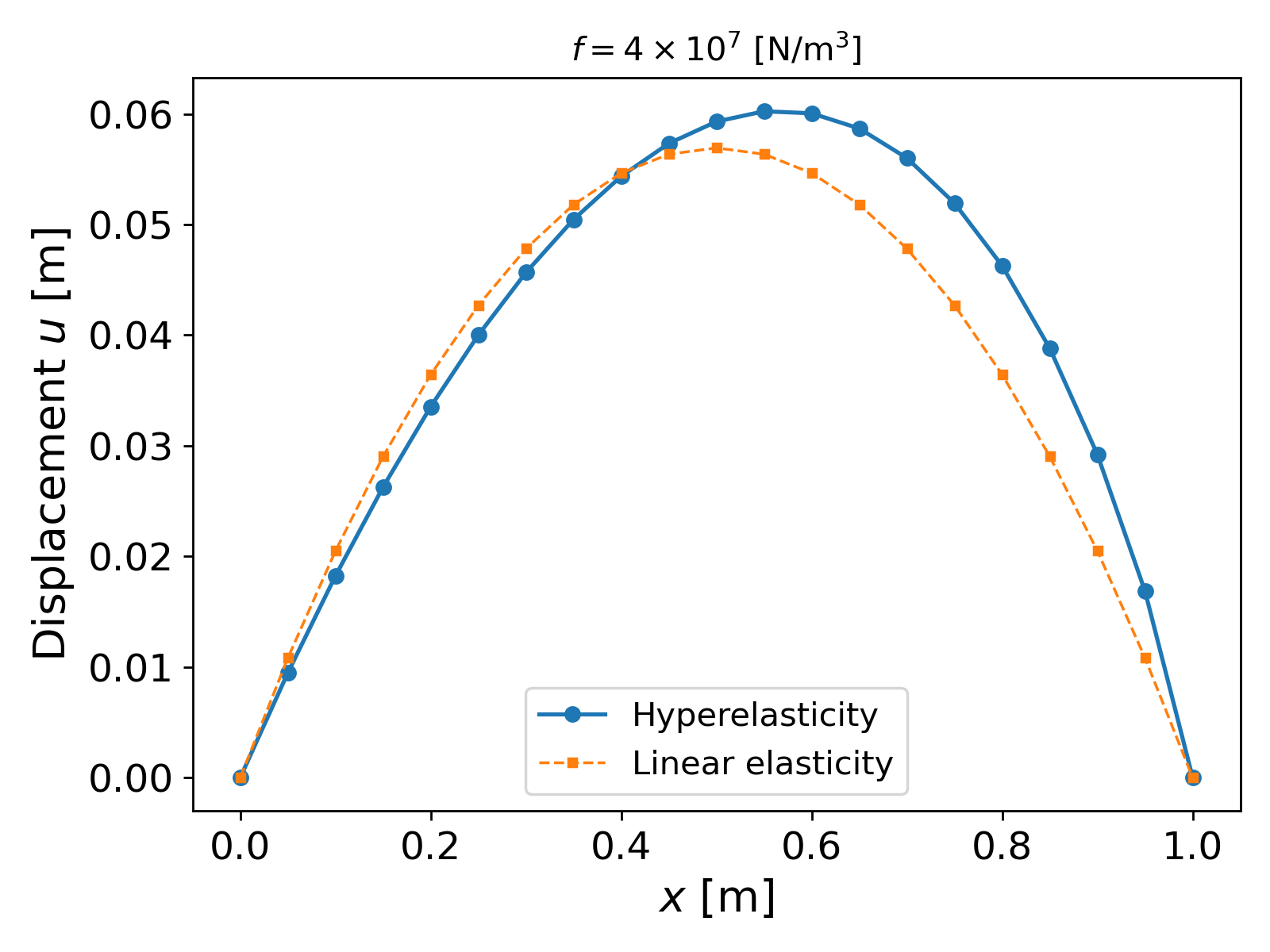
It can be observed from Fig. 3. that up to forces of O($10^6$), linear elasticity provides a good approximation and is quite close to the hyperelastic solution. For large magnitude loads, however, the difference in displacements becomes more apparent as seen in the right plot of Fig. 3. This is also consistent with the result in [Ciarlet’ 1988, Theorem 6.8-1] which provides an estimate of the difference of the linear elasticity and hyperelasticity displacements up to the norm of $f$.

Also, the linear elastic solution shows that the displacement profile achieves a maximum at the middle node $X = 0.5$, whereas the hyperelastic profile shows that the maximum displacement is more towards the $X = 0.6$ with higher displacement values as well.

On the solver side, Newton’s method performs well and converges within $2$ iterations when $f = 10^6$ and within $6$ iterations when $f = 4 \times 10^7$.

Robustness of Newton’s Method. We now investigate the robustness of Newton’s method to a different initial guess, which will help gauge the accuracy of our scheme and also help us implement a dynamic time dependent problem later on. Since the solution is close to a parabolic profile, we choose a non-zero initial guess $U^{(0)}(X) = 0.9X(1 - X)$ (the $0.9$ factor keeps the condition $F > 0$). The results are plotted in Fig. 4.

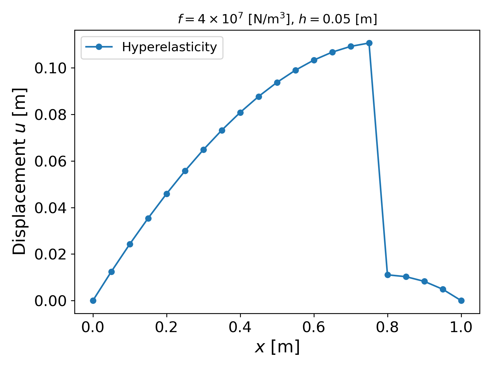
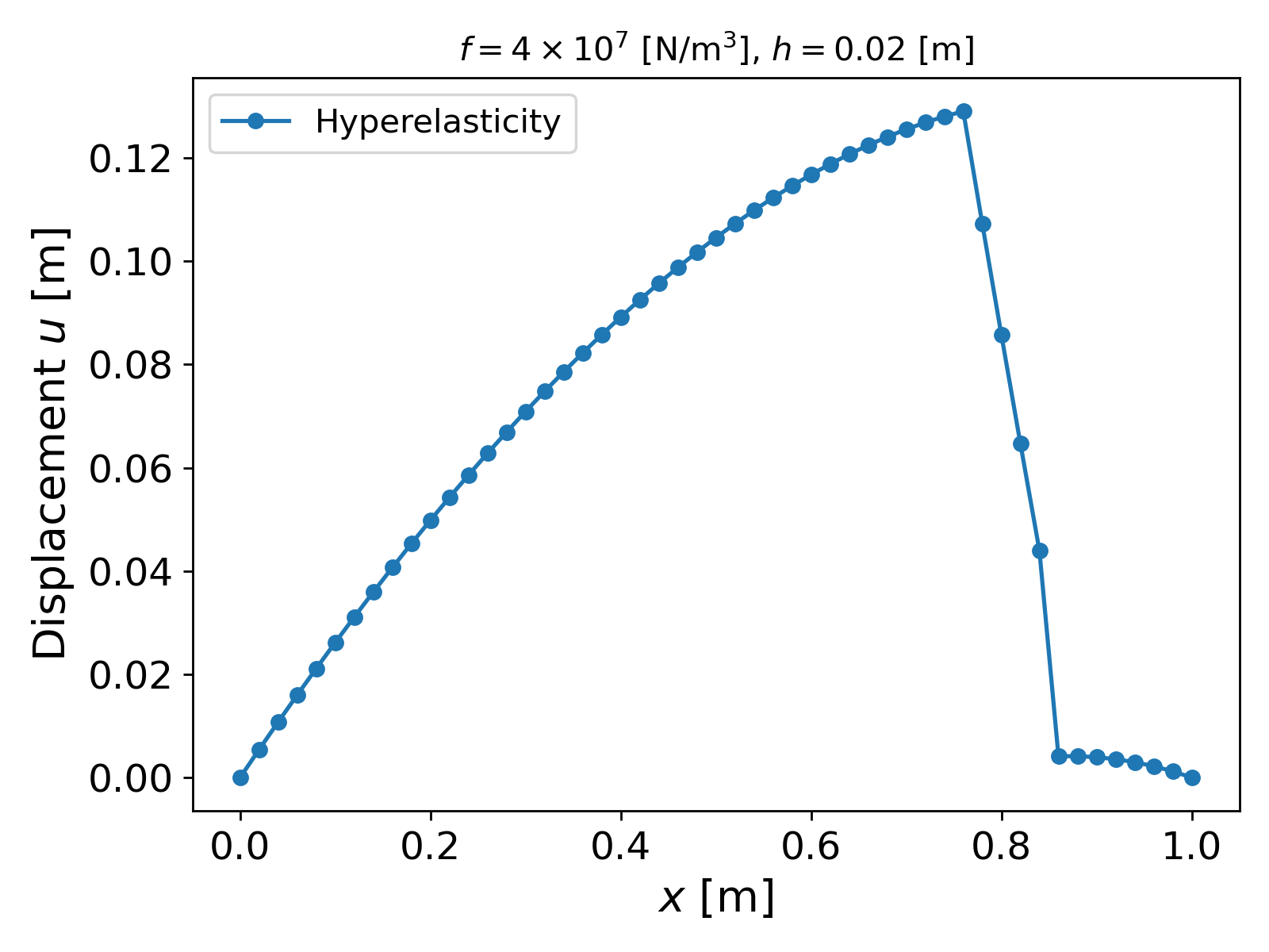
Things now take an interesting turn. The Newton solver converges, but the displacement profile is very different from what we obtained in Fig. 3. This is also an issue since the results in Fig. 4 are not entirely physical as the deformation gradient $F$ ceases to be positive, i.e., the deformation loses its orientation preservation property (see Fig. 7). Naturally, the first instinct is to refine the grid and see what happens, but to no avail. Fig. 4 also shows the solution profile for a refined grid, which does not look promising either.

The next step is to make sure that our numerical implementation is correct, and for that reason we also implement the St-Venant Kirchhoff hyperelastic system using FEniCS ¹⁰.

Results verification using FEniCS. We first verify our solution is using the initial guess $U^{(0)} = 0$, and then using $U^{(0)} = 0.9X(1-X)$. The results are shown in Fig. 5.

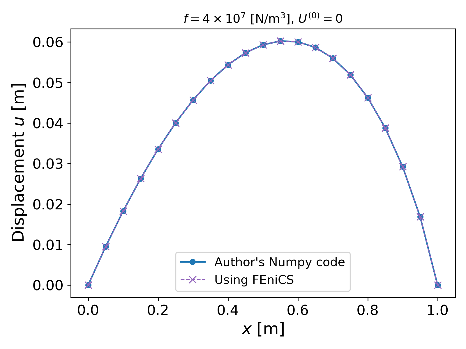
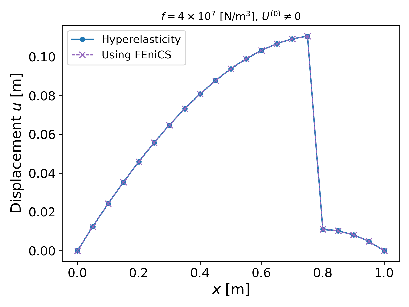
For both the cases, the solution profiles are almost identical and we achieve good agreement. This gives us more confidence in our implementation, and helps us to further investigate and identify the reason for this aberrant behavior of the nonlinear solver.

4. Issues with Well-Posedness: Non-uniqueness of Solution

From a numerical point of view (disregarding physical meaning of the solution), the results above highlight the lack of robustness of our nonlinear solver: we have convergence, but the solution profiles are not unique. Of course, uniqueness is the first thing to look at, and the reader may have noted that till now we have only spoken of existence and not uniqueness. Indeed, we now show that we can very well have situations with our St-Venant Kirchhoff system where multiple solutions exist.

We now proceed with constructing one such scenario. Consider the Dirichlet boundary conditions

Let $f = 0$, and let $E_Y > 0$ and $\nu \in (0, 0.5)$ be given. Consider the two solution profiles given by (see Fig. 6)

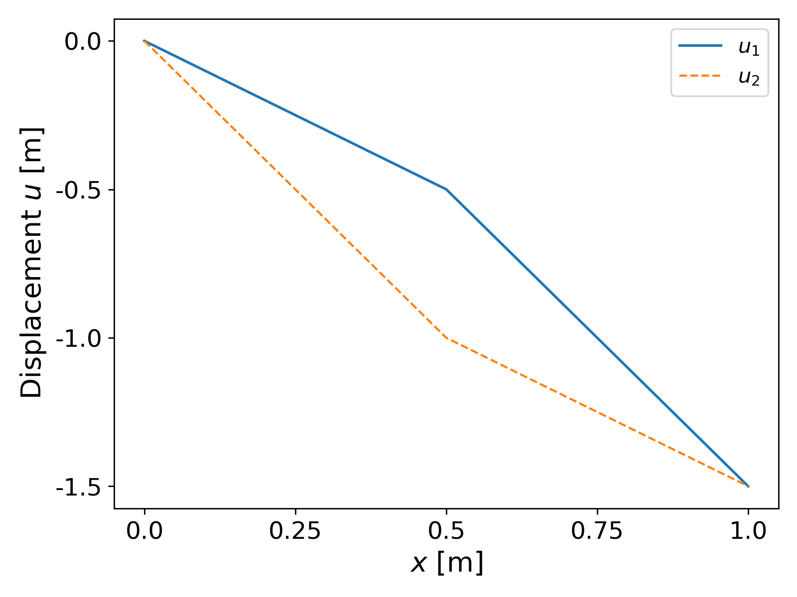
Clearly $u_1 \in H^1(\Omega)$ and $u_2 \in H^1(\Omega)$. Now by using the definition of $F = 1 + \frac{du}{dX}$ and $E = \frac{1}{2}\left(F^2 - 1 \right)$ and \eqref{eq:st_venant_fpks} we have

Since $u_1$ is piecewise linear, and

it can be easily verified that $T(u_1) = 0$. Similar case follows for $u_2$ and it holds that $T(u_2) = 0$. Thus the variational form \eqref{eq:discrete_weak_form} is satisfied for at least two different solutions, thereby providing non-uniqueness of the system.

Note. The reader may construct more such piecewise-linear displacement profiles by simply finding more roots of the polynomial

for any given constant $f \in \mathbb{R}$. In fact, similar profiles can be construced for the homogeneous Dirichlet boundary conditions as well by finding $\alpha_1, \alpha_2$ which satisfy $\alpha_1 \alpha_2 < 0$ for $f > 0$, $f$ small enough, for instance.

This helps explain the issue that we faced above, i.e., the Newton’s method has performed well, and it just probably converged to a different solution that was closer to the initial guess that was chosen. In fact, if we consider a coarse grid profile of what we have in Fig. 3 as the initial guess, then the solution converges to a similar profile for finer grids as well.

4.1. Lack of Orientation Preservation: $F < 0$

In the above discussion, another key aspect that we have implicitly assumed is that det$\nabla \phi = F > 0$. This means that the map $\phi$ remains injective and invertible (no two points in the reference configuration are mapped to the same point in the current configuration), providing some physical soundness to the solution. This, however, has not been enforced by us in the numerical implementation. Indeed, if we plot the deformation gradient $F$ for the examples above, it is clear that $F > 0$ ceases to hold true. This is shown in Fig. 7. for the case of $h = 0.02$ [m].

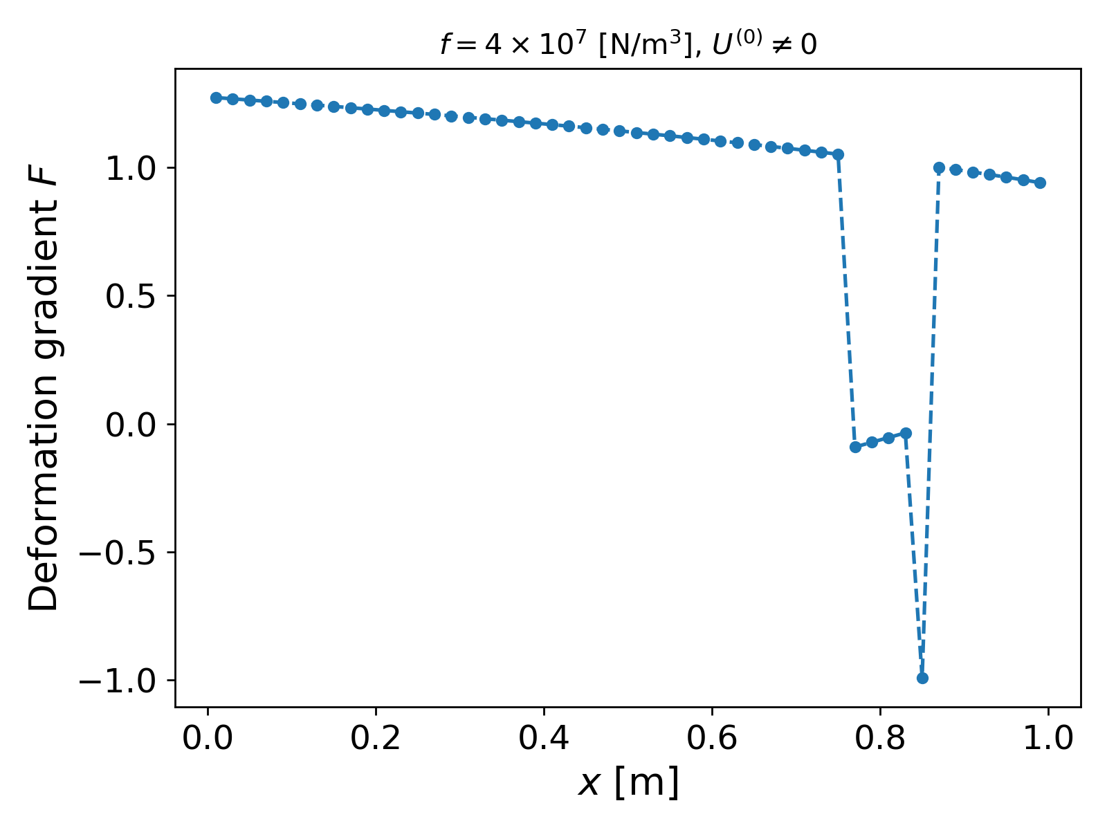
Thus, in the above examples, the deformation map $\phi$ loses its injectivity, which makes the results physically unsound as well. This is also what happens when $f$ becomes too large. Since orientation preservation is an important assumption and aspect of existence and uniqueness results, we will aim to potentially investigate and implement that in a future blog post.

Note. Whether enforcing $F > 0$ will solve the uniqueness issue, however, is another matter that has to be investigated. Take for example the non-unique solution profiles that were constructed above in Fig. 6. By a similar method, for some $f < 0$, $f$ small, we can find $\alpha_1, \alpha_2$ that solve \eqref{eq:polynomial_g} such that $\alpha_1, \alpha_2 \in (-1, 0)$ (since $g < 0$ in $(0, 1)$, and $g(0) = g(1) = 0$). Then, by considering a suitable Dirichlet boundary condition, we can construct similar displacement profiles which satisfy $\frac{du}{dX} \in \{\alpha_1, \alpha_2 \}$, but which would also satisfy $F = 1 + \frac{du}{dX} > 0$ since $\alpha_1, \alpha_2 > -1$. Thus, physically sound results might also require enforcing some necessary conditions on the boundary values as well.

Further Reading and Thoughts

The above exposition provides a brief (very brief!) introduction to the numerical aspect of solving hyperelasticity equations, in particular, to nonlinear mechanics. We considered the simplest form of materials, the St-Venant Kirchhoff material, owing to its simple expression, and demonstrated the challenges of Newton’s method insofar as non-uniqueness of the solution is concerned. One need not go as far as considering different intial guesses, as the author of this post has encountered issues and irregular solution profiles for $U^{(0)} = 0$ but for finer grids and for different $f$. Now we also note another issue, namely that the Jacobian may not always be invertible. Indeed, considering

it can be seen when $F_h \approx \sqrt{\frac{1}{3}}$ then $\mathcal{J}$ becomes singular. This highlights the importance of a good initial guess and robustness in general. The author of this post has also investigated fixed point iteration and line search methods, but to no remarkable avail: although the fixed point iteration avoids inverting the Jacobian, it is very slow owing to its linear convergence and may require posing the system as a contraction map. Moreover (now unsurprisingly due to non-uniqueness) with such methods convergence to irregular profiles as above was also observed.

The issue of solution converging to different profiles for different initial guesses can also be reproduced by simply chosing different grid sizes (as shown in Fig. 4). For example, for a zero intial guess, we have also observed different solution profiles for the same values of $f$ when varying $h$. The reason for this behaviour is also the same as above, i.e., non-uniqueness of solution. If, however, we already have a physically sound solution on a coarse grid, we may use that as an initial guess for a finer grid, which makes the solution converge to a similar profile as the coarse grid solution.

We plan to continue our investigation and consider higher dimensions and different methods and materials. That however, is the topic of a future blog post.

Code

The Author’s Numpy implementation is given below. The particular version of Numpy used is 1.26.4. Note that the code focuses on clarity of numerical implementation and might not be computationally very efficient, especially for finer grids.

# Script for 1D Hyperelasticity using St-Venant Kirchhoff materials.
# Author: Naren Vohra (NarenVohra1994@gmail.com).
# The script uses homogeneous Dirichlet boundary conditions and plots the displacement
# and deformation gradient when run.

import numpy as np
import matplotlib.pyplot as plt
import copy

################################
## Function definitions
################################

# Define dead load value
def f_fn(x):

    return 4e7

# Define initial guess
def U_init(x):

    U = np.zeros((M-1, 1))

    for j in np.arange(0, M-1, 1):

        #U[j] = x[j] * (1.0 - x[j]) * 0.9
        U[j] = 0.0

    return U

# Define Green strain tensor
def E(F):

    return 0.5 * (F * F  - 1.0)

# Define first Piola-Kirchhoff stress tensor and its gradient
def P(F, lambda_val, mu_val):

    return (lambda_val + 2.0 * mu_val) * F * E(F) 

def grad_P(F, lambda_val, mu_val):

    return (lambda_val + 2.0 * mu_val) * 0.5 * (3 * F * F  - 1)

# Compute residual using current displacement U
# Note that here we assume Dirichlet boundary conditions when computing deformation gradient F
def compute_residual(U, lambda_val, mu_val):

    R = np.zeros((M-1, 1))

    for i in np.arange(0, M-1, 1):
        if i == 0:
            F1 = (U[0] - 0.0)/h + 1.0       # Homogeneous Dirichlet boundary value
            F2 = (U[1] - U[0])/h + 1.0

            R[i] = P(F1, lambda_val, mu_val) * (1.0/h) * h - f_fn(xc[i]) * h * 0.5
            R[i] += P(F2, lambda_val, mu_val) * (-1.0/h) * h - f_fn(xc[i+1]) * h * 0.5

        elif i == M-2:
            F1 = (U[M-2] - U[M-3])/h + 1.0
            F2 = (0.0 - U[M-2])/h + 1.0     # Homogeneous Dirichlet boundary value

            R[i] = P(F1, lambda_val, mu_val) * (1.0/h) * h - f_fn(xc[i]) * h * 0.5
            R[i] += P(F2, lambda_val, mu_val) * (-1.0/h) * h - f_fn(xc[i+1]) * h * 0.5

        else:
            F1 = (U[i] - U[i-1])/h + 1.0
            F2 = (U[i+1] - U[i])/h + 1.0

            R[i] = P(F1, lambda_val, mu_val) * (1.0/h) * h - f_fn(xc[i]) * h * 0.5
            R[i] += P(F2, lambda_val, mu_val) * (-1.0/h) * h - f_fn(xc[i+1]) * h * 0.5

    return R

# Compute the Jacobian
def compute_jacobian(U, lambda_val, mu_val):

    J = np.zeros((M-1, M-1))

    for i in np.arange(0, M-1, 1):
        if i == 0:
            F1 = (U[0] - 0.0) / h + 1.0     # Homogeneous Dirichlet boundary value
            F2 = (U[1] - U[0]) / h + 1.0

            dP1 = grad_P(F1, lambda_val, mu_val).item()
            dP2 = grad_P(F2, lambda_val, mu_val).item()

            J[i][i] = (dP1 + dP2) * (1/(h*h)) * h
            J[i][i+1] = dP2 * (-1.0/(h*h)) * h

        elif i == M-2:
            F1 = (U[M-2] - U[M-3]) / h + 1.0 
            F2 = (0.0 - U[M-2]) / h + 1.0   # Homogeneous Dirichlet boundary value

            dP1 = grad_P(F1, lambda_val, mu_val).item()
            dP2 = grad_P(F2, lambda_val, mu_val).item()

            J[i][i] = (dP1 + dP2) * (1/(h*h)) * h
            J[i][i-1] = dP1 * (-1.0/(h*h)) * h

        else:
            F1 = (U[i] - U[i-1]) / h + 1.0
            F2 = (U[i+1] - U[i]) / h + 1.0

            dP1 = grad_P(F1, lambda_val, mu_val).item()
            dP2 = grad_P(F2, lambda_val, mu_val).item()

            J[i][i-1] = dP1 * (-1.0/(h*h)) * h
            J[i][i+1] = dP2 * (-1.0/(h*h)) * h
            J[i][i] =  (dP1 + dP2) * (1.0/(h*h)) * h

    return J

################################
## Main script
################################

# Elasticity parameters
# Young's modulus and Poisson's ratio
E_Young = 1e7
nu = 0.48

# Calculate Lamé parameters
lambda_val = E_Young * nu / ((1 + nu) * (1 - 2 * nu))
mu_val = E_Young / (2 * (1 + nu))

# Number of cells for spatial discretization and grid size
# Here we have assumed a domain (0, 1)
M = 20
h = 1.0/M

# Define cell faces (xf) and cell centers (xc)
xf = np.linspace(0, 1, M + 1)
xc = xf[0:-1] + h/2

# Newton's method parameters
max_it = 100        # Maximum iterations
tol_abs = 1.e-12    # Absolute tolerance
tol_rel = 1.e-14    # Relative tolerance
it = 0              # Current iteration

U = U_init(xf[1:-1])

# Start Newton's loop
while(it < max_it):

    # Compute residual
    R = compute_residual(U, lambda_val, mu_val)

    # Compute Jacobian
    J = compute_jacobian(U, lambda_val, mu_val)

    # Compute update
    deltaU = np.linalg.solve(J, -R)

    # Update solution after storing current iterate
    U_prev = copy.deepcopy(U)
    U += deltaU

    # Compute norms and check for convergence
    residual_norm = np.linalg.norm(R, ord = np.inf)
    deltaU_norm = np.linalg.norm(deltaU, ord = np.inf)

    if ((deltaU_norm < tol_rel) or (residual_norm < tol_abs)):
        print("---- ---- ---- ----")
        print(f"Converged in {it} iterations!")
        print(f"Maximum residual achieved {residual_norm}")
        print(f"Maximum difference of consecutive iterations achieved  {deltaU_norm}")
        print("---- ---- ---- ----")

        break

    # Update
    it += 1

    if (it == max_it):
        print(f"No convergence!")
        print(f"Maximum residual achieved {residual_norm}")

        break

# Add homogeneous Dirichlet boundary values to displacement vector
U = np.insert(U, 0, 0)
U = np.append(U, 0)

# Now solve for linear elasticity
# Set up linear elasticity stiffness matrix
Alin = np.zeros((M-1, M-1))

for j in np.arange(0, M-1, 1):

    if j == 0:
        Alin[j][j] = (lambda_val + 2.0 * mu_val) * 2.0 * (1/h)
        Alin[j][j+1] = (lambda_val + 2.0 * mu_val) * -1.0 * (1/h)
    elif j == M-2:
        Alin[j][j] = (lambda_val + 2.0 * mu_val) * 2.0 * (1/h)
        Alin[j][j-1] = (lambda_val + 2.0 * mu_val) * -1.0 * (1/h)
    else:
        Alin[j][j] = (lambda_val + 2.0 * mu_val) * 2.0 * (1/h)
        Alin[j][j-1] = (lambda_val + 2.0 * mu_val) * -1.0 * (1/h)
        Alin[j][j+1] = (lambda_val + 2.0 * mu_val) * -1.0 * (1/h)

# Calculate right hand side dead load vector
Flin = np.zeros((M-1, 1))

for j in np.arange(0, M-1, 1):
    Flin[j] = f_fn(xc[j]) * h * 0.5 * 2.0

# Solve system
Ulin = np.linalg.solve(Alin, Flin)

# Add homogeneous Dirichlet boundary values to displacement vector
Ulin = np.insert(Ulin, 0, 0)
Ulin = np.append(Ulin, 0)

# Plot results
# Plot displacements
fig = plt.figure()

plt.plot(xf, U, linewidth = 1.5, marker = "o", markersize = 5.0, label = "Hyperelasticity")
plt.plot(xf, Ulin, linewidth = 1.0, linestyle = "--", marker = "s", markersize = 3.0, label = "Linear elasticity")

plt.xlabel(r"$x$ [m]", fontsize = 16)
plt.ylabel(r"Displacement $u$ [m]", fontsize = 16)

plt.xticks(fontsize = 14)
plt.yticks(fontsize = 14)

plt.legend(loc = "best", fontsize = 12)

plt.tight_layout()


# Plot deformation gradient
# Calculate deformation gradient 
F = np.zeros((len(xc), 1))

for j in np.arange(0, M, 1):
    F[j] = (U[j+1] - U[j])/h + 1.0

Flin = np.zeros((len(xc), 1))

for j in np.arange(0, M, 1):
    Flin[j] = (Ulin[j+1] - Ulin[j])/h + 1.0

# Plot
fig = plt.figure()

plt.plot(xc, F, linewidth = 1.5, marker = "o", linestyle = "--", markersize = 4.0, label = "Hyperelasticity")
plt.plot(xc, Flin, linewidth = 1.0, linestyle = "--", marker = "s", markersize = 3.0, label = "Linear elasticity")

plt.xlabel(r"$x$ [m]", fontsize = 16)
plt.ylabel("Deformation gradient $F$", fontsize = 16)

plt.xticks(fontsize = 14)
plt.yticks(fontsize = 14)

plt.legend(loc = "best", fontsize = 12)

plt.tight_layout()
plt.show()
# Script ends

References

Philippe G. Ciarlet, Mathematical Elasticity: Volume 1: Three-dimensional Elasticity, 1988, Elsevier Science Publishers. ↩ ↩2 ↩3 ↩4 ↩5 ↩6 ↩7
I. H. Shames and F. A. Cozzarelli, Elastic and Inelastic Stress Analysis, 1997, Taylor and Francis Group. ↩
J. Bonet and R. D. Wood, Nonlinear Continuum Mechanics for Finite Element Analysis, 1997, Cambridge University Press. ↩ ↩2
J. Tinsley Oden, Existence Theorems for a Class of Problems in Nonlinear Elasticity, 1979, Journal of Mathematical Analysis and Applications. ↩
W. Rudin, Principles of Mathematical Analysis, 1976, McGraw-Hill, Inc., 3rd edition. ↩
S. C. Brenner and L. R. Scott, The Mathematical Theory of Finite Element Methods, 2008, Springer, 3rd Edition. ↩
C. T. Kelley, Iterative Methods for Linear and Nonlinear Equations, 1995, Society for Industrial and Applied Mathematics. ↩
Charles R. Harris et al., Array programming with NumPy, 2020, Springer Science and Business Media (LLC). ↩
Young’s Modulus of Elasticity – Values for Common Materials, Poisson’s Ratio – Definition, Values for Materials, and Applications Engineering Toolbox, retrieved in 2026. ↩
I. A. Baratta et al., DOLFINx: The next generation FEniCS problem solving environment, 2023. ↩