
An Attempt Towards a Robust St-Venant Kirchhoff Type Model in Hyperelasticity
Date:
1. Introduction
In this blog post, we continue towards building a robust solver for the St-Venant Kirchhoff hyperelastic model. In our previous blog post, we delved into the challenges that arise when solving for
\[\label{eq:governing_system} -\nabla \cdot T(u) = f \text{ in } \Omega,\]in a 1D setting, and now we investigate the challenges that arise in a 2D setting. In particular, we are interested in investigating how the St-Venant Kirchhoff model behaves in a well-known benchmark case: the incompressible block compression scenario; see Fig. 1 for an illustration of the domain and problem.
As we have already observed in our previous blog post, for large compressive forces the St-Venant Kirchhoff model struggles to converge to a solution, or it may converge to a solution that is not orientation preserving, i.e., a non-physical solution, and hence is not the best model to simulate the block compression scenario. Indeed, the St-Venant Kirchhoff model is usually best to simulate scenarios involving small strains 1. The convergence issue is further aggravated as the model for finer grid sizes, which are needed to avoid the effect of locking when using low order finite elements.
In this post, we are interested to see how far we can push the St-Venant Kirchhoff model, and if there is a way to make modifications which can help us better approximate and capture displacement profiles under large forces and for fine grids. To this end, we focus on building a new St-Venant Kirchhoff type model by adding a linear term which can help us approximate large displacements while avoiding the above challenges. Our motivation comes from an apriori knowledge of the lack of well-posedness of the system and we introduce physical “stiffness” which helps us solve this issue to some extent and also allows the new model to capture displacement profiles under large forces and on finer grids.
2. Details of the Computational Solver
Following the notation we set up in our previous blog post, we recall the St-Venant Kirchhoff model
\[\label{eq:st_venant_kirchhoff_def} T = F\left[ \lambda \text{tr}(E)I + 2\mu E \right],\]where $\lambda$ and $\mu$ are Lamé parameters. We concern ourselves with only the reference configuration $\Omega$ in 2D, i.e., $\Omega \subset \mathbb{R}^2$. We consider the system \eqref{eq:governing_system} with mixed boundary conditions
\[\label{eq:mixed_bc} u = 0 \text{ on } \partial \Omega_D, \; T n = t_N \text{ on } \partial \Omega_N,\]where $t_N$ [Pa] is the given traction which is assumed to be smooth enough (we are mostly concerned with constant values here), and the Dirichlet boundary condition on $u = (u_1, u_2)$ is equivalent to
\[u_1 = 0, \; u_2 = 0 \text{ on } \partial \Omega_D.\]2.1. Numerical Discretization
The variational problem associated with the above system \eqref{eq:governing_system}-\eqref{eq:mixed_bc} is given as follows: we seek $u_h \in V_h$ such that 1
\[\label{eq:variational_form} \int_\Omega T(u_h) : \nabla \phi_h = \int_\Omega f \cdot \phi_h + \int_{\partial \Omega_N} t_N \cdot \phi_h, \; \forall \phi_h \in V_h,\]where
\[V_h \subset (H^1_D(\Omega))^2 = \{ \phi_h \in (H^1(\Omega))^2 \; | \; \phi_h = 0 \text{ on } \partial \Omega_D \}\]is the finite dimensional subspace of Q1 bilinear elements on $\Omega_h$. To avoid ambiguity due to notation, we highlight that in \eqref{eq:variational_form}, the basis elements $\phi_i : \mathbb{\Omega}_h \rightarrow \mathbb{R}^2$ are vector-valued functions, and
\[\nabla \phi_h = \begin{bmatrix} \frac{\partial {\phi_h}_1}{\partial X_1} \; \frac{\partial {\phi_h}_1}{\partial X_2} \\ \frac{\partial {\phi_h}_2}{\partial X_1} \; \frac{\partial {\phi_h}_2}{\partial X_2} \end{bmatrix}, \; \phi_h = \begin{bmatrix} {\phi_h}_1 \\ {\phi_h}_2 \end{bmatrix}.\]For any $\phi_h \in V_h$, the $H^1$ semi-norm $\vert \cdot \vert_2$ is defined as
\[\big| \phi_h \big|_2^2 = \sum_{i, j=1}^{2} \int_\Omega \Big| \frac{\partial {\phi_h}_i}{\partial X_j} \Big|^2\]Using the Poincaré inequality, $\vert \cdot \vert_2$ becomes a norm on $(H^1_0(\Omega))^2$.
2.2. Nonlinear Solver: Newton’s Method
We now recall some details of Newton’s method, which we use to solve the nonlinear system of equations resulting from \eqref{eq:variational_form}. Letting $\{ \phi_i \}$ denote the $N$ basis elements for $V_h$, we consider the residuals defined as
\[\label{eq:nonlinear_residual} \mathcal{T}_i (u_h) = \int_\Omega T(u_h): \nabla \phi_i - \int_{\partial \Omega_N} tN \cdot \phi_i - \int_\Omega f \cdot \phi_i, \; \forall 1 \leq i \leq N.\]and thus we seek a solution $U = \left[U_1 \; U_2 \; \dots \; U_N \right]^T \in \mathbb{R}^{N}$ to
\[\label{eq:nonlinear_eq} \mathcal{T}(U) = 0,\]where $u_h = \sum_{i=1}^N U_i \phi_i$ and $\mathcal{T} = [\mathcal{T}_1 \; \mathcal{T}_2 \; \dots \mathcal{T}_N]^T$.
The Newton’s method to solve for \eqref{eq:nonlinear_eq} gives the following algorithm: starting from $u^{(0)}_h \in V_h$, perform the update 2
\[\label{eq:newton_update} U^{(m)} = U^{(m-1)} - {\mathcal{J}^{(m-1)}}^{-1} \mathcal{T}^{(m-1)},\]where $\mathcal{T}^{(m-1)} = \mathcal{T}(U^{(m-1)})$ is the residual at $U^{(m-1)}$ and $\mathcal{J}^{(m-1)} = \left(\nabla_U \mathcal{T}\right) (U^{(m-1)})$ is the Jacobian of $\mathcal{T}$ (here $\nabla_U$ denotes the gradient with respect to $U$).
We now investigate the properties of the Jacobian $\mathcal{J}$ which will help us select an appropriate linear solver to compute its inverse $\mathcal{J}^{-1}$ when performing the update \eqref{eq:newton_update}.
2.2.1. Symmetric Property of the Jacobian
We begin by simplifying the Jacobian. Note that from \eqref{eq:nonlinear_residual}, we have for any given $U$
\[\label{eq:jacobian_def} \mathcal{J}_{i, j} = \frac{\partial \mathcal{T}_i}{\partial U_j} (U) = \int_{\Omega} \frac{\partial T(u_h)}{\partial U_j} : \nabla \phi_i\]Let us simplify the expression \eqref{eq:jacobian_def}. First, note that by definition we have
\[F(u_h) = I + \nabla u_h = I + \sum_{i=1}^{N} U_i \nabla \phi_i,\]and thus
\[\label{eq:F_gradient} \frac{\partial F}{\partial U_j} = \nabla \phi_j, \; \forall 1 \leq j \leq N.\]Now, since $E = \frac{1}{2}\left(F^T F - I \right)$, we have from \eqref{eq:F_gradient}
\[\label{eq:E_gradient} \frac{\partial E}{\partial U_j} = \frac{1}{2} \left(\nabla \phi_j^T F + F^T \nabla \phi_j \right), \; \forall 1 \leq j \leq N.\]Using \eqref{eq:F_gradient} and \eqref{eq:E_gradient} in \eqref{eq:st_venant_kirchhoff_def} we get
\[\frac{\partial T}{\partial U_j} = \lambda \left[ \text{tr}(E) \nabla \phi_j + \frac{1}{2} \text{tr}\left(\nabla \phi_j^T F + F^T \nabla \phi_j \right) \right] +\] \[\mu \left[2 \nabla \phi_j E + F \left(\nabla \phi_j^T F + F^T \nabla \phi_j \right) \right].\]Thus, we have the expression
\[\label{eq:jacobian_def_2} \mathcal{J}_{i, j} = \int_\Omega \lambda \left[ \text{tr}(E) \nabla \phi_j : \nabla \phi_i + \frac{1}{2} \text{tr}\left(\nabla \phi_j^T F + F^T \nabla \phi_j \right) \left(F : \nabla \phi_i \right) \right] +\] \[\mu \left[2 \left(\nabla \phi_j E\right) : \nabla \phi_i + \left(F \left(\nabla \phi_j^T F + F^T \nabla \phi_j \right) \right):\nabla \phi_i \right]. \nonumber\]We now prove an that the Jacobian is symmetric.
Lemma 2.2.1.1. The Jacobian $\mathcal{J}$ defined by \eqref{eq:jacobian_def_2} is symmetric.
Proof. We consider individual terms in the integrand of \eqref{eq:jacobian_def_2}. Note that the term
\[\text{tr}(E) \nabla \phi_j : \nabla \phi_i\]is trivially symmetric (by interchanging $i$ and $j$). We now consider the other terms.
Note that for any two square matrices $A$ and $B$, the double contraction operator is defined as
\[A : B = \text{tr} (A^T B) = \text{tr} (A B^T),\]and $\text{tr}(AB) = \text{tr}(BA)$.
We now consider the term
\[\label{eq:second_term} \text{tr} \left(\nabla \phi_j^T F + F^T \nabla \phi_j \right) \left(F : \nabla \phi_i \right).\]First note that using the above identities $\text{tr}\left(\nabla \phi_j^T F \right) = \text{tr}\left( F^T \nabla \phi_j \right)$. Also, we can rewrite \eqref{eq:second_term} as
\[2 \text{tr} \left(F^T \nabla \phi_j \right) \text{tr} \left(F^T \nabla \phi_i \right),\]which is symmetric in $i$ and $j$. Thirdly, we consider the term
\[\left(\nabla \phi_j E \right) : \nabla \phi_i,\]which we rewrite as
\[\label{eq:third_term_2} \text{tr} \left( F^TF \nabla \phi_j^T \nabla \phi_i \right) - \text{tr} \left(\nabla \phi_j^T \nabla \phi_i \right) = \text{tr} \left( F^TF \nabla \phi_j^T \nabla \phi_i \right) - \nabla \phi_i : \nabla \phi_j.\]Further, using commutativity, we can rewrite \eqref{eq:third_term_2} as
\[\text{tr} \left(\nabla \phi_i F^TF \nabla \phi_j^T \right) - \nabla \phi_i : \nabla \phi_j = F \nabla \phi_i^T : F \nabla \phi_j^T - \nabla \phi_i : \nabla \phi_j,\]which is symmetric in $i$ and $j$. Fourthly, and finally, we consider the term
\[\left(F \left(\nabla \phi_j^T F + F^T \nabla \phi_j \right) \right):\nabla \phi_i,\]which we rewrite as
\[\label{eq:fourth_term} \text{tr} \left(F^T \nabla \phi_j F^T \nabla \phi_i \right) + \text{tr} \left(\nabla \phi_j^T F F^T \nabla \phi_i \right).\]Using the definition of $:$ we can rewrite \eqref{eq:fourth_term} as
\(\text{tr} \left(F^T \nabla \phi_j F^T \nabla \phi_i \right) + F^T \nabla phi_j : F^T \nabla \phi_i.\) By the commutativity of trace and $:$, the symmetry in $i$ and $j$ follows. This proves that $\mathcal{J}$ is symmetric.
□
The above lemma guides us in choosing a linear solver to compute the inverse $\mathcal{J}^{-1}$. We choose a solver that leverages the symmetric property of $\mathcal{J}$, but we cannot naively expect too much out of, say, Conjugate Gradient since $\mathcal{J}$ need not be positive definite. Thus, we proceed with minimal residual (MINRES) method to handle our symmetric indefinite Jacobian 3. However, note that the above lemma does not prove that $\mathcal{J}$ is invertible, and proving that would require investigating the bilinear operator associated with each Newton update, which we do not discuss here.
2.2. Anticipated Challenges
In our previous post, we exemplified the issues of existence and uniqueness for simple scenarios. This led to, for example, (i) lack of convergence of computational solver for finer grid sizes, or (ii) convergence to different solution profiles for different initial guesses in the nonlinear solver (Newton’s method). Indeed, there is no reason for us to not expect such challenges in 2D (or 3D). Moreover, a very well known challenge in mechanics is expected to arise given our choice of the low order Q1 finite elements: locking 3. Locking occurs for incompressible materials, and is defined as the inability of the computational solver to provide an accurate solution profile (displacements) for coarse meshes. For linear elasticity, locking can be explained by loss of coercivity of the associated bilinear form when $\frac{\lambda}{\mu} \rightarrow \infty$, which leads to large error for a given grid size $h$ 4.
Locking is well-studied in literature, and there exists multiple formulations (eg. mixed, weak Galerkin etc.) that are known to reduce the effect of locking. Or simply, one may use Q2 elements which, in our experience as well, reduces locking. In our experiments, however, since we work with finer grids to test the robustness of our model, we do not encounter locking to a high degree when using Q1 elements.
3. Numerical Results
We now investigate the performance of our computational solver in physical scenarios. We implement the computational solver using the finite element library deal.II 5. We consider the MINRES solver as the linear solver when computing the solution $\delta U = \mathcal{J}^{-1} \mathcal{T}$. The absolute and relative tolerances to which we solve the system are $\epsilon_{ns, abs} = 10^{-8}$ and $\epsilon_{ns, rel} = 10^{-10}$. The MINRES algorithm stops when a tolerance of $\epsilon_{ls} = 10^{-8} \times \lVert \mathcal{T} \rVert_2$ is achieved.
3.1. Clamped Bar Under Dead Load
We begin with the clamped bar under a constant force scenario from our previous blog post. Extending into 2D, we now consider $\Omega = (0, 1) \times (0, 0.4)$ [m $^2$]. The boundary conditions are
\[u = 0 \text { on } x = 0, 1, \; T n = 0 \text{ on } y = 0, 0.4.\]The Young’s modulus is $E_Y = 10^7$ [Pa] and the Poisson ratio is $\nu = 0.48$ [-]. For an external force of $f = 4 \times 10^7$ [N / m $^3$], our computational solver does not converge, and hence we choose a smaller force of $f = 3 \times 10^6$. The results are shown in Fig. 2 for a uniform grid size of $0.025 \times 0.025$ [m $^2$] (i.e. $h = 0.025$).
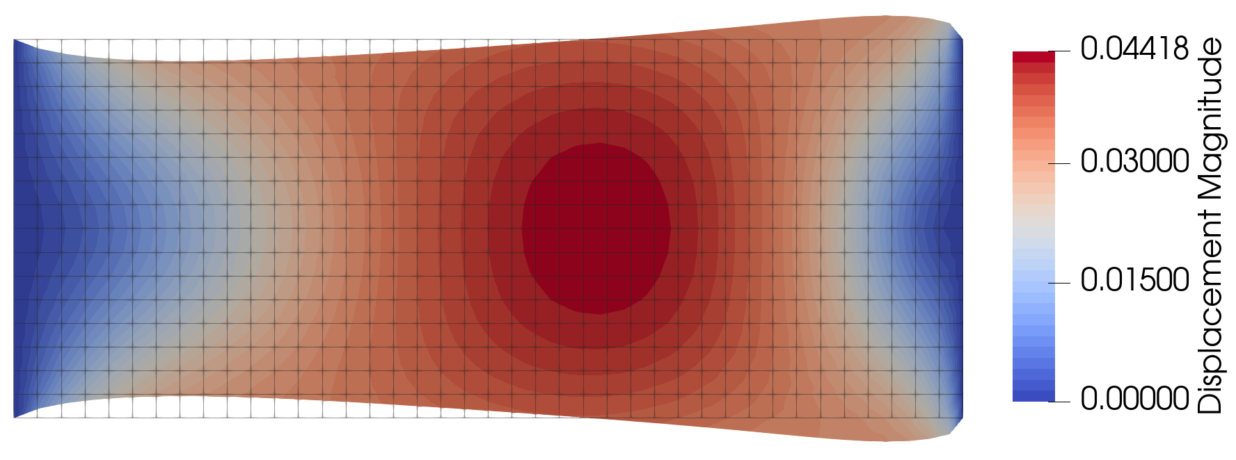
The profile shows the bar deformed with more mass accumulating towards the right boundary. We also tabulate the performance of the computational solver in Tab. 1. It can be observed that the number of nonlinear and linear iterations increase as the mesh is refined, and we quickly reach a stage of no convergence for a small enough grid size $h$, i.e., for a fine grid. No locking was observed in this example, which is unsurprising since the material is not highly incompressible (owing to $\nu = 0.48$).
| Grid size | #DoFs (N) | Convergence? | NS iter. | LS iter. |
|---|---|---|---|---|
| 0.1 | 110 | Yes | 5 | 305 |
| 0.05 | 378 | Yes | 6 | 961 |
| 0.025 | 1394 | Yes | 9 | 3339 |
| 0.0125 | 5346 | No | - | - |
It is also noted that when the force $f$ is increased further, the computational solver does not converge (or exhibits non-physical scenarios associated with det$(F) < 0$). Moreover, the LS iter. increase proportionally to the size of the system, i.e., the number of DoFs N, which is not ideal as we will encounter the “curse of dimensionality” as we move into 3D. Although, this we can hope to resolve to some extent with a suitable preconditioner.
3.2. Incompressible Block Compression
We now proceed with investigating the performance of the computational solver on an incompressible block compression scenario as depicted in Fig. 1. The benchmark is well-known and is taken from 6 among other references, and is usually simulated using a Neo-Hookean model. The material parameters are chosen from 7. In particular, the Young’s modulus is taken to be $E_Y = 240.565 \times 10^6$ [Pa] and the Poisson ratio is taken to be $\nu = 0.4999$ [-].
Re-selecting $t_N$ to obtain convergence. We consider traction vector as $t_N = (-4 \times 10^8, 0)$ [Pa] as in 7, however, our computational solver does not converge. To obtain convergence, we reduce the traction magnitude to $t_N = -7 \times 10^7$ (after trial and error with different grid sizes). The results are shown in Fig. 3 for different grid sizes.
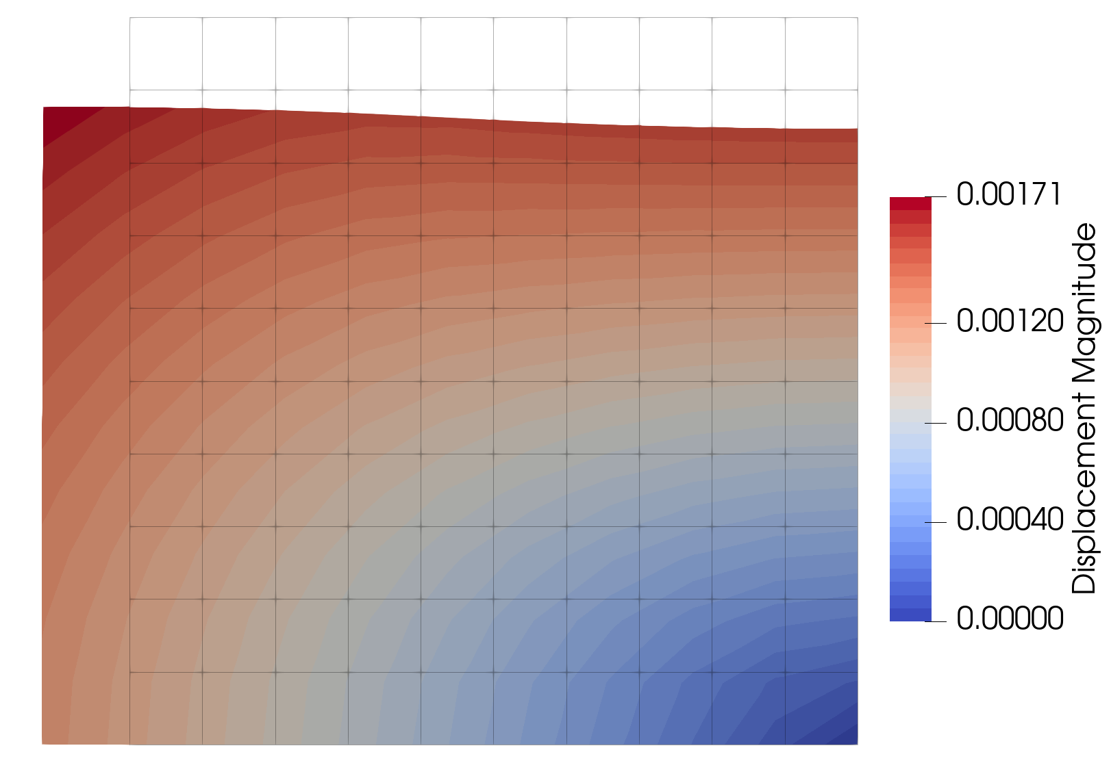
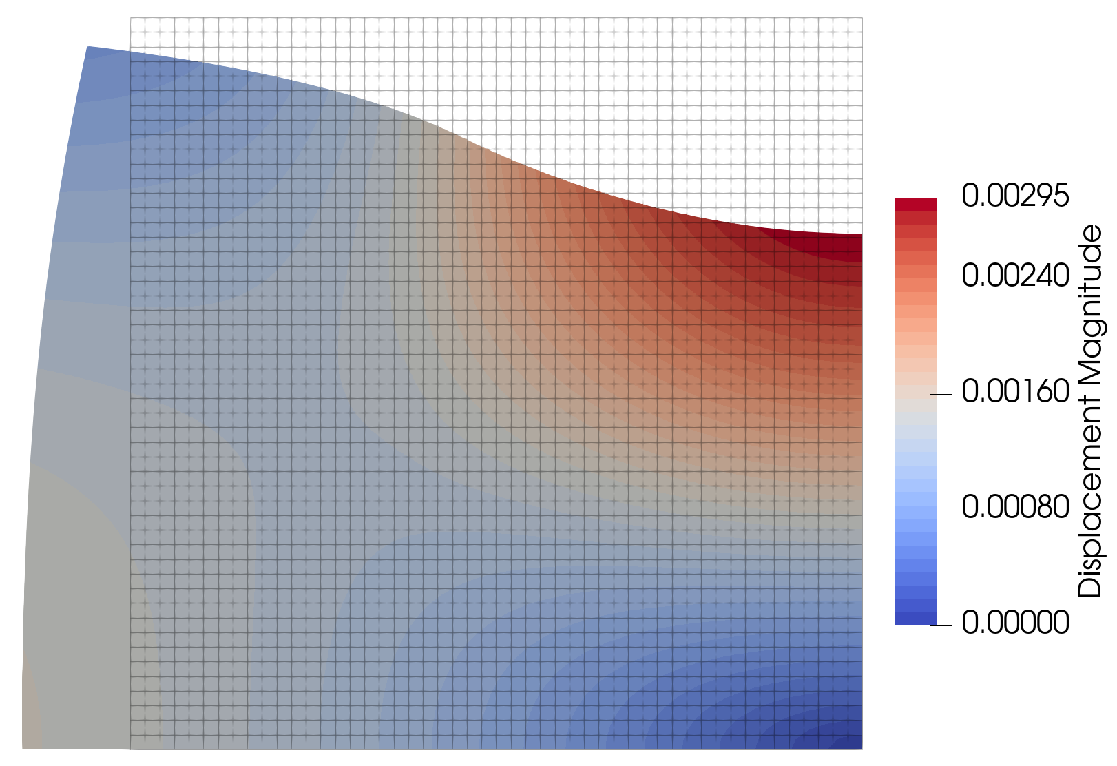
We can now observe some severe locking taking place in the solution. Indeed, the deformed configurations look very different and the maximum displacement magnitude of the two profiles differs by a factor of ~$1.7$. Moreover, the maximum vertical displacement we are able to achieve is $2.95$ [mm] at point $(10, 10)$, whereas the results reported in 7 are close to $6$ [mm], a big difference. On the solver side, for grid size $h = 1$ and $h = 0.02$ convergence is achieved in NS iter. 6 and LS iter. 3922, and NS iter. 14 and LS iter. 138170, numbers which can definitely take major improvements.
We note that in both the examples above our model and solver struggles to converge for large $f$ or $t_N$, values which may have led to convergence in 1D. Moreover, even for small $f$ or $t_N$, if we refine the grid sufficiently we reach a stage where we either get a non-physical solution, or our solver does not converge, behaviour that was also observed in 1D in our previous blog post discussion. We now work on addressing this issue by introducing a new parameter in the St-Venant Kirchhoff model.
4. Introducing a New Model
The above examples (and the discussion in our previous blog post) show how poorly the St-Venant Kirchhoff model performs for typical physical scenarios, on the physical and computational side. In particular, for large forces or traction, the solver does not converge, or the solution converges to an non-physical profile (such as where det$(F) < 0$), issues which we now try to address through the lack of well-posedness of the St-Venant Kirchhoff model. We now work towards improving the model through a stabilizing term to see if we can attempt to have well-posedness in some form.
Note. The discussion below is not found on any experimental data, and is just to explore how a material responds to a “modified” St-Venant Kirchhoff type model. We try to provide mathematical rigour on some clear assumptions, which, however, are not guaranteed to hold true for all physical scenarios, although we have seen agreeable improvement in some examples.
Let $\gamma > 0$ be a parameter. We list the exact dependence of $\gamma$ later, and here we note that the units of $\gamma$ are [Pa]. Consider now the modified constitutive law
\[\label{eq:modified_law} \widetilde{T}(u) = T(u) + \gamma \nabla u,\]where we have now introduced an diffusion term with the material (when we take the divergence of \eqref{eq:modified_law}). The reader may link this to the concept of artificial diffusion to improve the stability of numerical methods, but physically this terms adds extra stiffness for large displacement valuesr That is, we now expect a stiffer response from the material, but only enough so that we obtain physically sound solution profiles when external forces are large.
We now proceed towards obtaining a numerical solution to the system arising from \eqref{eq:modified_law}. The variational form now becomes: find $u_h \in V_h$ such that
\[\label{eq:modified_variational_form} \int_\Omega T(u): \nabla \phi_h + \gamma \int_\Omega \nabla u_h : \nabla \phi_h = \int_{\partial \Omega_N} t_N \cdot \phi_h + \int_\Omega f \cdot \phi_h, \; \forall \phi_h \in V_h,\]where now it is understood that the traction boundary condition is applied as $\widetilde{T} n = t_N$.
Existence of solution to Newton’s update. We note that if $\gamma$ is large enough then the Jacobian associated with $\widetilde{T}$ becomes symmetric positive definite (SPD) since
\[\widetilde{\mathcal{J}} = \mathcal{J} + \gamma \mathcal{A},\]where
\[\mathcal{A}_{i, j} = \int_\Omega \nabla \phi_i : \nabla \phi_j\]is an SPD matrix. Thus for large $\gamma$, the eigenvalues of $\widetilde{\mathcal{J}}$ can be made positive since $\mathcal{A}$ has positive eigenvalues (it is SPD) and $\mathcal{J}$ has real eigenvalues (it is symmetric). This further guarantees existence of a unique update $\delta U$ in each Newton iteration.
Well-posedness in 1D. We now provide an outline of a proof of well-posedness for the new model. Let us consider the variational form \eqref{eq:modified_variational_form} with homogeneous Dirichlet boundary conditions for simplicity and clarity of exposition. We also now denote by $V_h \subset H_0^1(\Omega)$ the finite dimensional subspace of piecewise-linear functions which vanish on $\partial \Omega$. Rewriting \eqref{eq:modified_variational_form} using a nonlinear operator $a : V_h \rightarrow V_h’$, where $V_h’$ is the dual of $V_h$, the variational form becomes: we seek $u_h \in V_h$ such that
\[a(u_h)(\phi_h) = S(\phi_h),\]where
\[\label{eq:modified_problem} a(u_h)(\phi_h) = \int_\Omega T(u_h): \nabla \phi_h + \gamma \int_\Omega \nabla u_h : \nabla \phi_h,\]and $S \in V_h’$ is defined as
\[\label{eq:S_def} S(\phi_h) = \int_\Omega f \cdot \phi_h.\]We now investigate properties of the operator $a$. In particular, we are interested in establishing some form of coercivity and monotonicity which will guarantee the existence of a unique solution using the Minty-Browder’s theorem [Ciarlet’ 2013, Theorem 9.14-1] 8. That, however, is not a trivial task, and instead we will prove the properties in 1D while also making use of a cut-off operator to compute the tensors $F$ and $E$ as
\[F_{C} = 1 + C\left(\frac{d u}{dX} \right), E_C = \frac{1}{2} \left(F_C^2 - 1 \right),\]where
\[C \left(\frac{du}{dX} \right) = \begin{cases} \frac{d u_h}{d X}; & \text{ if } |\frac{d u_h}{d X}| < C_0, \\ C_0 \frac{d u_h}{d X_j} \left(|\frac{d u}{d X}|\right)^{-1}; & \text{ otherwise}, \end{cases}\]and the constant $C_0 > 0$ is taken to be large enough. That is, the cut-off operator $C : \mathbb{R} \rightarrow \mathbb{R}$ is defined as
\[C(x) = \begin{cases} x; & \text{ if } |x| < C_0, \\ C_0 \frac{x}{|x|}; & \text{ otherwise}. \end{cases}\]such that
\[\label{eq:C_bounds} \big|C(x) \big| \leq C_0, \; \big|C \big| \leq |x|, \; \forall x \in \mathbb{R}.\]Note that $C$ is also Lipschitz continuous, and we denote the Lipschitz constant by $L_C$.
Now, define
\[T_C(u) = \frac{\left(\lambda + 2\mu \right)}{2} F_C \left(E_C^2 - 1 \right),\]and consider the following variational formulation: we seek $u_h \in V_h$ such that
\[\label{eq:modified_var_form} a_C(u_h)(\phi_h) = S(\phi_h), \forall \phi_h \in V_h,\]where
\[\label{eq:modified_aC} a_C(u_h)(\phi_h) = \int_\Omega T_C(u_h) \frac{du_h}{dX} \frac{d\phi_h}{dX}.\]and $S$ is defined as in \eqref{eq:S_def}, i.e.,
\[S(\phi_h) = \int_\Omega f \phi_h.\]Note on the cut-off operator. The idea of the cut-off operator is that for a large enough $C_0$, the system \eqref{eq:modified_aC} is close to \eqref{eq:modified_problem}, and hence a numerical implementation of the cut-off operator is unnecessary for large $C_0$. However, we rely on the cut-off operator for formal analysis and an existence result as proved below. The cut-off operator is used in literature in other problems as well: see for example 9 for an application in thermo-poroelastic settings.
We now state an existence result making use of the concepts of monotonicity, coercivity, and hemicontinuity of operators. For a brief introduction and definitions, see also the monograph 10. Note that since $V_h$ is a finite dimensional Hilbert space, it is reflexive and separable.
Theorem 4.1. Fix $h > 0$ and $C_0 > 0$. Then, the operator $a_C : V_h \rightarrow V_h’$ is strictly monotone, hemicontinuous, and coercive for a large enough $\gamma > 0$. Thus $\exists$ a unique solution to \eqref{eq:modified_var_form} for a smooth enough $f$.
Proof. First note that since $\frac{du_h}{dX}$ is a piece-wise constant function, we can rewrite
\[a_C(u_h)(\phi_h) = \frac{\left(\lambda + 2\mu \right)}{2} \int_\Omega g_1\left( C\left(\frac{du}{dX} \right) \right) \phi_h,\]where the polynomial $g_1 : \mathbb{R} \rightarrow \mathbb{R}$ is defined as $g_1(\alpha) = \alpha(\alpha + 1)(\alpha + 2)$. Now, let $u_h, v_h \in V_h$. To prove that $a_C$ is hemicontinuous, we need to show that
\[B(t) = a_C(u_h + t v_h)(\phi_h)\]is continuous on an interval $(-t_0, t_0), t_0 > 0$ for any $u_h, v_h, \phi_h \in V_h$. This follows easily since if $\{ t_n \}$ is a sequence such that $t_n \rightarrow 0$ then
\[\label{eq:step-1_proof} B(t_n) - B(0) = \frac{\left(\lambda + 2\mu \right)}{2} \int_\Omega \left[ g_1\left( C\left(\frac{du}{dX} + t_n \frac{dv_h}{dX} \right) \right) - g_1 \left(C \left(\frac{du_h}{dX} \right) \right) \right] \frac{d\phi_h}{dX}\] \[+ \gamma t \int_\Omega \frac{dv_h}{dX} \frac{d \phi_h}{dX}. \nonumber\]The second term in \eqref{eq:step-1_proof} can be bounded by Hölder’s inquality since $v_h, \phi_h \in H^1_0(\Omega_h)$, and hence $\rightarrow 0$ as $t \rightarrow 0$. For the first term, note that since $g$ is a polynomial, and $(x - y)$ divivides $(x^m - y^m)$ for any $x, y \in \mathbb{R}$ and $m \in \mathbb{Z}$, $m > 0$, we can write $g(x) - g(y) = (x - y) g_2(x, y)$, for some polynomial $g_2 : \mathbb{R} \times \mathbb{R} \rightarrow \mathbb{R}$. Thus, we can rewrite the first term in \eqref{eq:step-1_proof} as
\[A_0 = \frac{\left(\lambda + 2\mu \right)}{2} \int_\Omega \left[ g\left( C\left(\frac{du}{dX} + t_n \frac{dv_h}{dX} \right) \right) - g \left(C \left(\frac{du_h}{dX} \right) \right) \right] \frac{d\phi_h}{dX}\] \[= \frac{\left(\lambda + 2\mu \right)}{2} \int_\Omega \left[ C\left(\frac{du}{dX} + t_n \frac{dv_h}{dX} \right) - C \left(\frac{du_h}{dX} \right) \right] g_2\left(C\left(\frac{du_h}{dX}\right), C \left(\frac{dv_h}{dX}\right) \right) \frac{d\phi_h}{dX} \nonumber\]By the Lipschitz continuity of $C$, and using the boundedness of $C$, we have that $A_0 \rightarrow 0$ as $t \rightarrow 0$. Thus, $B(t)$ is hemicontinuous at $t = 0$.
Now we work towards the montononicity of $a_C$. We have
\[\label{eq:step0_proof} a_C(u_h)(u_h - v_h) - a_C(v_h)(u_h - v_h)\] \[= \frac{\left(\lambda + 2\mu \right)}{2} \int_\Omega \left[ g_1\left(C\left( \frac{du_h}{dX} \right) \right) - g_1\left(C\left( \frac{dv_h}{dX} \right) \right) \right] \left(\frac{du_h}{dX} - \frac{dv_h}{dX} \right) + \nonumber\] \[\gamma \int_\Omega \left(\frac{du_h}{dX} - \frac{dv_h}{dX} \right)^2. \nonumber\]Using the factorization above, we can rewrite \eqref{eq:step0_proof} as
\[\label{eq:step1_proof} a_C(u_h)(u_h - v_h) - a_C(v_h)(u_h - v_h)\] \[= \frac{\left(\lambda + 2\mu \right)}{2} \int_\Omega g_2\left(C\left(\frac{du_h}{dX}\right), C \left(\frac{dv_h}{dX}\right) \right) \left(C\left( \frac{du_h}{dX} \right) - C\left( \frac{dv_h}{dX} \right) \right) \left(\frac{du_h}{dX} - \frac{dv_h}{dX} \right) \nonumber\] \[+ \gamma \int_\Omega \left(\frac{du_h}{dX} - \frac{dv_h}{dX} \right)^2. \nonumber\]Now, by using the first inequality in \eqref{eq:C_bounds} and its Lipschitz continuity we can bound the first term in \eqref{eq:step1_proof}
\[A_1 = \frac{\left(\lambda + 2\mu \right)}{2} \int_\Omega g_2\left(C\left(\frac{du_h}{dX}\right), C \left(\frac{dv_h}{dX}\right) \right) \left(C\left( \frac{du_h}{dX} \right) - C\left( \frac{dv_h}{dX} \right) \right) \left(\frac{du_h}{dX} - \frac{dv_h}{dX} \right)\]by
\[\label{eq:step2_proof} \big|A_1 \big| \leq \frac{C_1 \left(\lambda + 2\mu \right)}{2} \int_\Omega \Bigg|\left(C\left( \frac{du_h}{dX} \right) - C\left( \frac{dv_h}{dX} \right) \right) \Bigg| \Bigg|\frac{du_h}{dX} - \frac{dv_h}{dX} \Bigg|\] \[\leq \frac{C_1 L_C \left(\lambda + 2\mu \right)}{2} \int_\Omega \Bigg|\frac{du_h}{dX} - \frac{dv_h}{dX} \Bigg|^2, \nonumber\]where $C_1 = C_1(C_0) = O(C_0^2)$ is some constant. Thus, we have from \eqref{eq:step2_proof} and using the triangle inequality
\[\label{eq:step3_proof} a_C(u_h)(u_h - v_h) - a_C(v_h)(u_h - v_h) \geq \left[\gamma - \frac{C_1 L_C \left(\lambda + 2\mu \right)}{2} \right] \big| u_h - v_h \big|_2^2.\]It can be observed that the RHS of \eqref{eq:step4_proof} is positive for a large enough $\gamma$. This proves that $a_c$ is stricitly montotone.
Similarly, we can prove the coercivity of $a_C$ by observing that since
\[\label{eq:step4_proof} a_C(u_h)(u_h) = \frac{\left(\lambda + 2\mu \right)}{2} \int_\Omega g\left( C\left( \frac{du_h}{dX} \right) \right) \frac{du_h}{dX} + \gamma \big| u_h \big|_2^2,\]we can bound the first term in \eqref{eq:step4_proof}
\[A_2 = \frac{\left(\lambda + 2\mu \right)}{2} \int_\Omega g\left( C\left( \frac{du_h}{dX} \right) \right) \frac{du_h}{dX}\]by using the inequalities in \eqref{eq:C_bounds} as
\[\big|A_2 \big| \leq \frac{(1 + C_0)(2 + C_0) \left(\lambda + 2\mu \right)}{2} \int_\Omega \Bigg| \frac{du_h}{dX} \Bigg| \Bigg| \frac{du_h}{dX} \Bigg| =\] \[\frac{(1 + C_0)(2 + C_0) \left(\lambda + 2\mu \right)}{2} \big| u_h \big|_2^2. \nonumber\]Thus we have
\[\label{eq:step5_proof} \frac{a_C(u_h)(u_h)}{\big| u_h \big|_2} \geq \left[\gamma - \frac{(1 + C_0)(2 + C_0) \left(\lambda + 2\mu \right)}{2} \right] \big| u_h \big|_2.\]Since the RHS of \eqref{eq:step5_proof} $\rightarrow \infty$ as $\vert u_h \vert_2 \rightarrow \infty$ for large enough $\gamma$, the coercivity of $a_C$ is also established. The result follows with the application of the Minty-Browder theorem.
□
The above theorem can be extended to higher dimensional settings as well, and provides us with well-posedness of our discretized modified problem.
Note. Perhaps the biggest (if not one of the biggest) problems with the above approach is that the parameter $\gamma$ depends on the grid size $h$. This means that for a fixed $\gamma$, if we keep refining the mesh, we will eventually land an ill-posed problem, where the computational solver will not converge and we can expect the same challenges as the St-Venant Kirchhoff model. This is duly noted, and is an interesting hard issue to solve, but in our regime of numerical results we don’t face much of an issue. We may think of $\gamma$ as a parameter that helps obtain a physically sound displacement profile for large compressive forces, and a parameter that we may fine tune if we know apriori the grid scales that we are dealing with.
5. Testing Our New Model: Numerical Results Revisited
We are now ready to test our new model on the physical scenarios discussed above. We begin by returning to the 1D clamped bar scenario as in our previous blog post to highlight the importance of well-posedness as proved above and see if we indeed have any improvement in the robustness of the solver.
5.1. 1D Clamped Bar Revisited
We now study the simple 1D clamped bar example to understand the performance of our new model compared with the St-Venant Kirchhoff model. We follow the same parameters and tolerances as mentioned in our previous blog post, and consider different grid sizes and initial guesses.
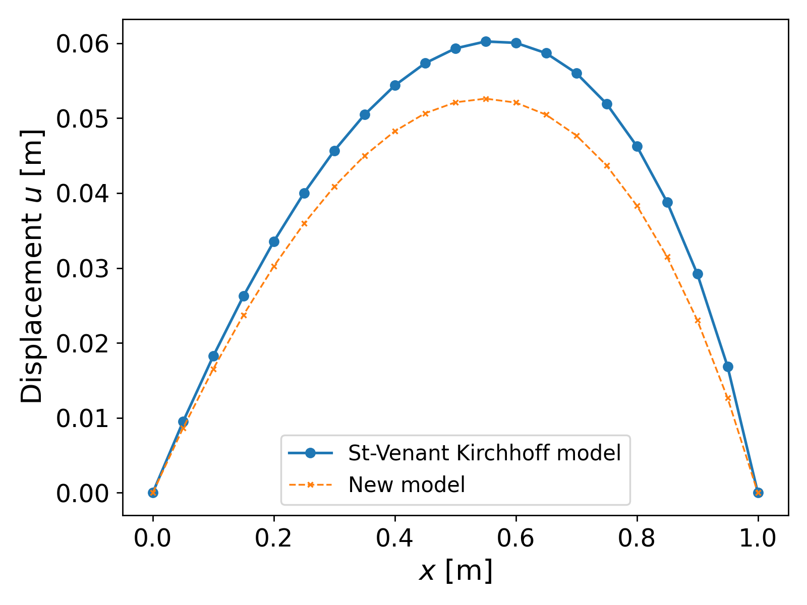
Scenario results with new model. We first simulate the scenario using grid size $h = 0.05$ [m] and by choosing $\gamma = 10^7$ [Pa]. The results are shown in Fig. 4.
Robustness testing. As discussed in our previous blog post, the 1D clamped bar example was not robust with the choice of a different initial guess $U^{(0)}$ or if we refine the grid too much when $f$ is large. We now test these aspects of robustness with our new modified model as in \eqref{eq:modified_law}. The results are shown in Fig. 5 and Fig. 6 below.
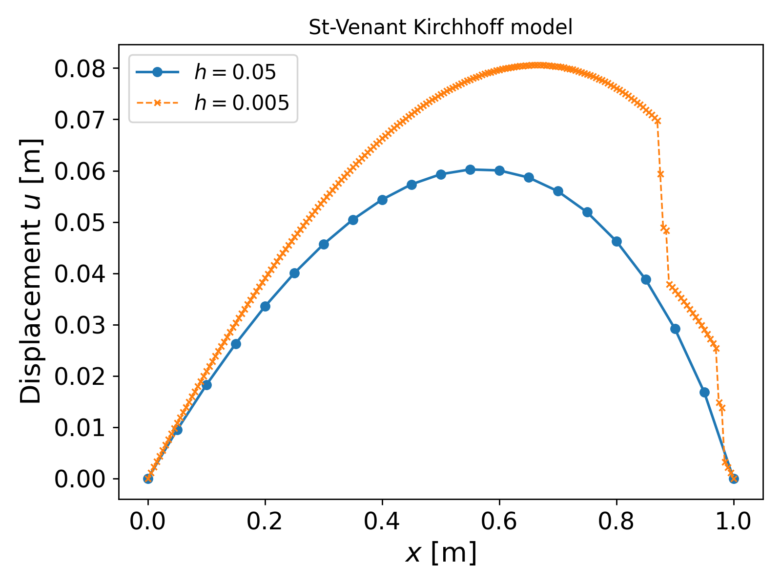
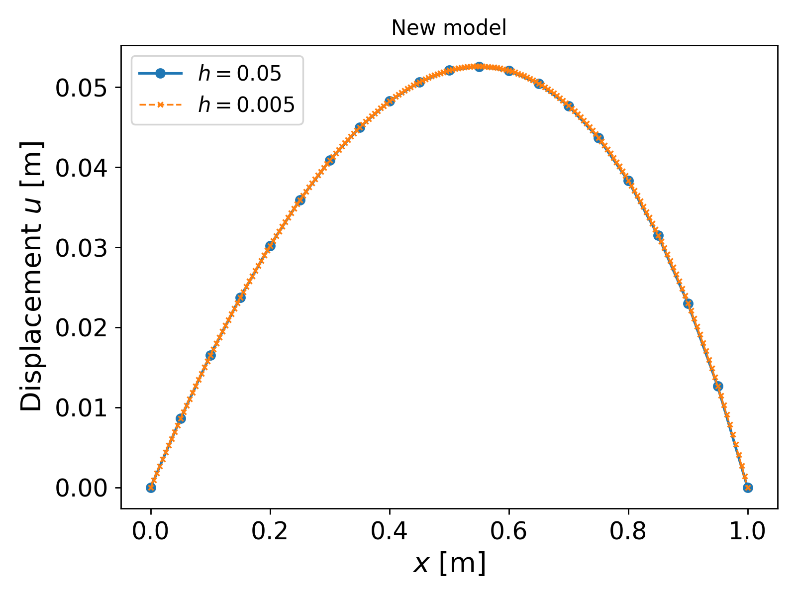
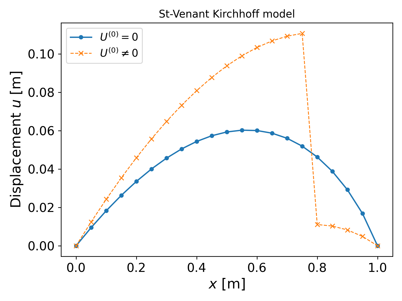
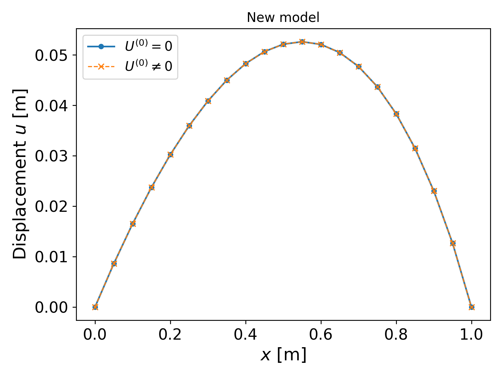
Performance summary. Let us now discuss the performance of the model and the computational solver. On the physical side, as expected, the material response is much more stiffer, resulting in smaller displacements for the new model. On the computational side, there is good improvement, and the results are tabulated in Tab. 2. In particular, we observe convergence of the solver for finer grids and different initial guesses, behaviour that was not observed when using the St-Venant Kirchhoff model.
| Case | St-Venant Kirchhoff NS iter. | New model NS iter. |
|---|---|---|
| Grid size h = 0.05 (Initial guess zero) | 6 | 5 |
| Grid size h = 0.005 (Initial guess zero) | 123 | 5 |
| Initial guess zero (Grid size h = 0.05) | 6 | 5 |
| Intial guess non-zero (Grid size h = 0.05) | 10 | 8 |
We also note that for smaller $\gamma$, the difference between the St-Venant Kirchhoff model and our new model is less (as expected), and consequently convergence issues also arise.
2D results. We now revisit the example above in 2D with $f = 4 \times 10^7$ and $\gamma = 1.55 \times 10^7$. The displacment profile is shown in Fig. 7 for a grid size of $0.0125 \times 0.0125$ [m $^2$] (which led to no-convergence for the St-Venant Kirchhoff model in our discussion above).
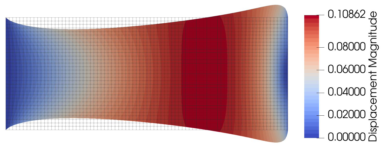
Unlike before, the solver now converges in NS iter. 11 and LS iter. 4653, and the maximum displacement magnitude is more than twice what it was in Fig. 2.
5.2. Incompressible Block With New Model
We are now in a position to provide the numerical results for the incompressible block scenario as above. We use $h = 0.05$ [mm] and $\gamma = 4 \times 10^8$ [Pa] (after some trial and error) for $t_N = 4 \times 10^8$. The results are shown in Fig. 8 below.
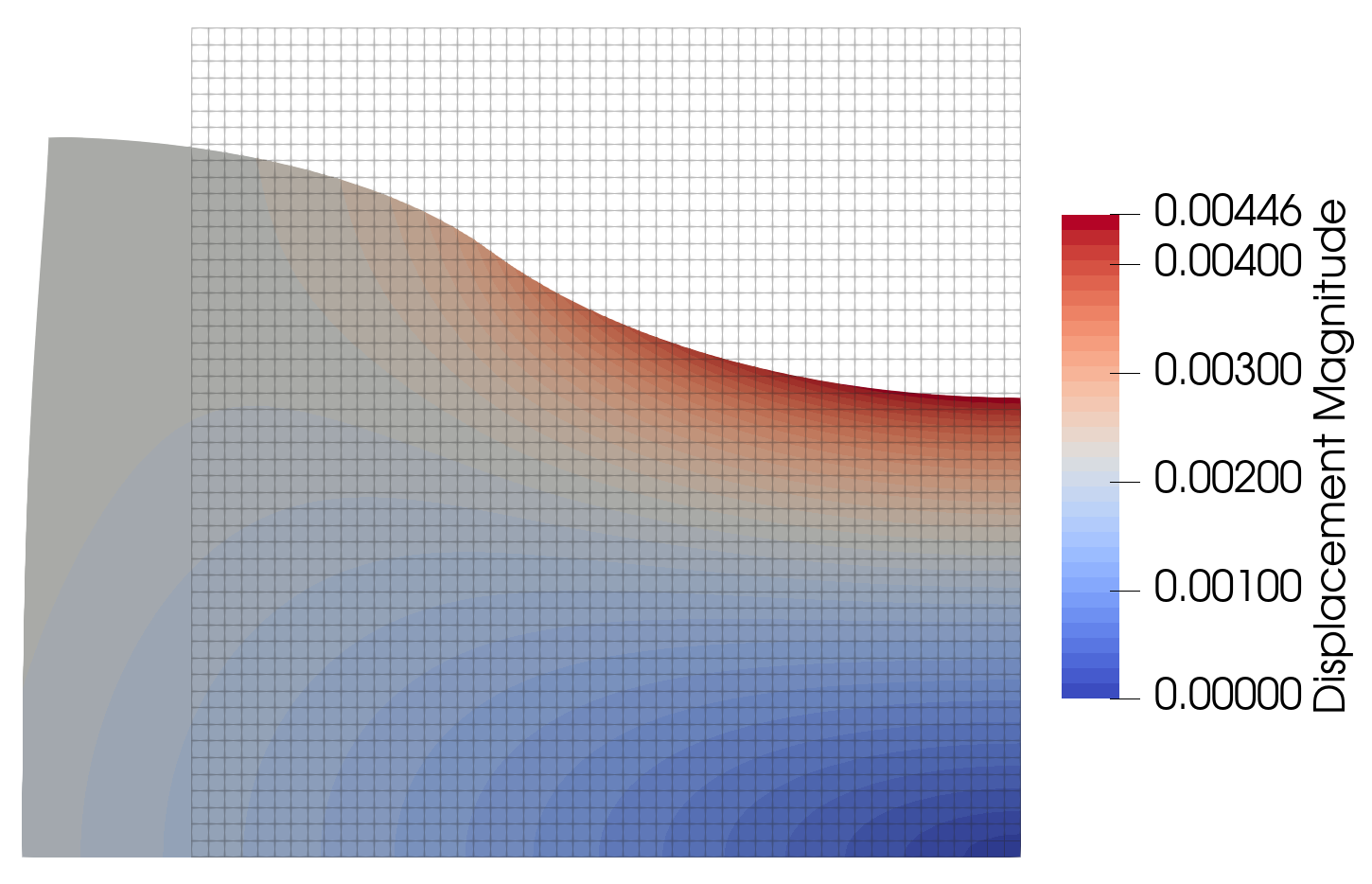
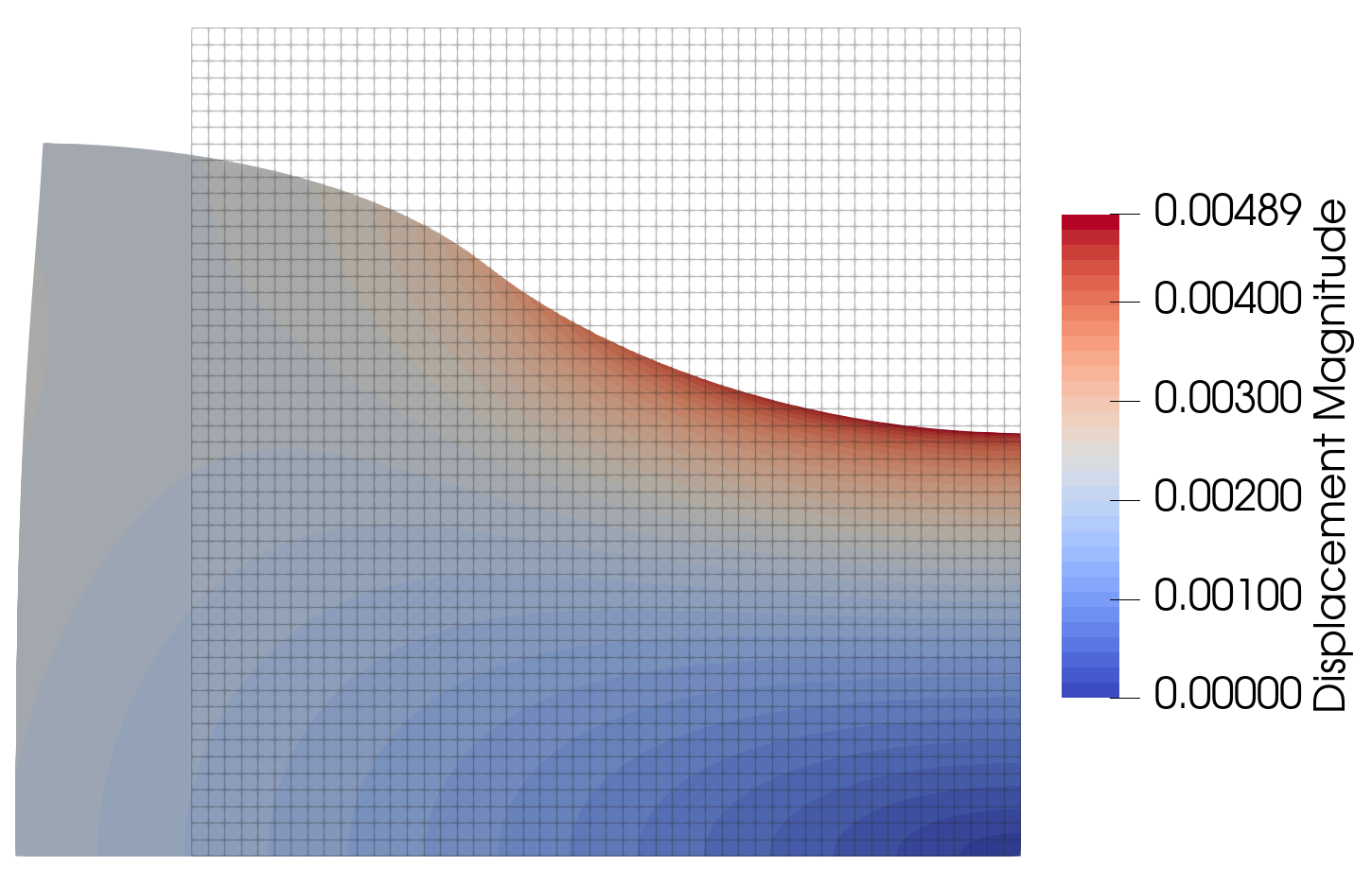
Fig. 8 (left) shows a much better displacement profile with a maximum value of 4.46 [mm], better than the values reported previously in Fig. 3, although still short of the benchmark values reported in 7. The NS iter. in this case are 13 and the LS iter. are 78411.
Sensitivity to $\gamma$. The model is expectedly sensitive to $\gamma$. A small $\gamma$ means we tend towards the St-Venant Kirchhoff model, and a large $\gamma$ means the material responds very stiffly. We attempt to increase the maximum displacement in the incompressible block scenario by varying $\gamma$. Indeed, after some more trial and error, it was observed that when $\gamma = 3.819 \times 10^8$, the maximum displacement improves to 4.89 [mm]; the profile is shown in Fig. 7 (right). In this case, the NS iter. taken are 21 and the LS iter. is 143151.
To conclude the above numerical results, we note that we are able to obtain physical displacement profiles for grid sizes and forces that the St-Venant Kirchhoff model could provide for. This is consistent with the well-posedness that we can hope to achieve with our new model for a large enough $\gamma$.
Further Reading and Thoughts
The above discussion provides an attempt at improving the physical and computational aspect of the St-Venant Kirchhoff model under large compressive forces. Although the new model introduced above is not found on any experimental data, we successfully demonstrate how the modification can help us achieve better results with improved performance, particularly by obtaining agreeable physical displacement profiles under large forces as opposed to the St-Venant Kirchhoff model which does not converge under the same forces. As highlighted, however, it should be noted that the new model does not inherently address the fundamental issue of the St-Venant Kirchhoff model which is that the stored energy function $W(F) \rightarrow 0$ as det$(F) \rightarrow 0$. Indeed, the stored energy of the new model is
\[\widetilde{W}(F) = \frac{\lambda}{2} \text{tr}(E)^2 + \mu \text{tr}(E^2) + \frac{1}{2}\left( \text{tr}(F^TF) - \text{tr}(F) \right),\]which, too, does not provide any resistance to det$(F) \rightarrow 0$ and will face the same issues as the St-Kirchhoff Venant model for large forces.
Moreover, a major drawback is that the parameter $\gamma$ depends on the space $V_h$, i.e., on the grid size $h$ for model and performance improvements, and we also cannot hope that $\gamma$ is dimension invariant: for example, if a particular $\gamma$ value gives good results in 2D, it may still require fine-tuning in 3D. Another issue is that for large $\gamma$ and for small forces or traction, the material response is too stiff which would result in very small and inaccurate displacements. To address this, a more versatile parameter could be a monotnone $\gamma = \gamma(u)$ which may still be able to provide coercivity and monotonicty of the operator associated with $\widetilde{T}$ (provided we may impose something like $\gamma(0) = 0$ and Lipschitz continuity), and would slowly introduce stiffness as $u$ increases with increasing $f$ or $t_N$. That, however, would be a topic for a future blog post.
References
Philippe G. Ciarlet, Mathematical Elasticity: Volume 1: Three-dimensional Elasticity, 1988, Elsevier Science Publishers. ↩ ↩2
Michael Ulbrich, Semismooth Newton Methods for Variational Inequalities and Constrained Optimization Problems in Function Spaces, 2011, Mathematical Optimization Society and the Society for Industrial and Applied Mathematics. ↩
D. Braess, Finite Elements: Theory, Fast Solvers, and Applications in Elasticity Theory, 2007, Cambridge University Press. ↩ ↩2
Alexandre Ern, Jean-Luc Guermond, Theory and Practice of Finite Elements, 2004, Springer. ↩
Daniel Arndt et al., The deal.II library, Version 9.7, Journal of Numerical Mathematics, 2025. ↩
Reese et al.’, A New Stabilization Technique For Finite Elements in Non-linear Elasticity, 1999, International Journal for Numerical Methods in Engineering, 44. ↩
Bayat et al.’, Numerical evaluation of discontinuous and nonconforming finite element methods in nonlinear solid mechanics, 2018, Computational Mechanics. ↩ ↩2 ↩3 ↩4
Philippe G. Ciarlet, Linear and Nonlinear Functional Analysis with Applications, 2013, SIAM. ↩
Brun et al.’, Monolithic and splitting solution schemes for fully coupled quasi-static thermo-poroelasticity with nonlinear convective transport, 2020, Computers and Mathematics with Applications. ↩
Ralph Showalter, Monotone Operators in Banach Space and Nonlinear Partial Differential Equations, 1997, American Mathematical Society. ↩